Valuing a Convertible Bond-Derivative Pricing in Python

In a previous post, we presented a theoretical framework for pricing convertible bonds and preferred shares.  We also provided an example of pricing a convertible bond in Excel. In this installment, we present an example of pricing a convertible bond in Python.

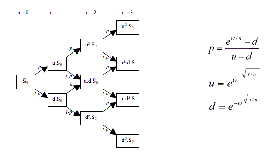
Recall that a convertible bond (or preferred share) is a hybrid security, part debt, and part equity. Its valuation is derived from both the level of interest rates and the price of the underlying equity. Several convertible bond pricing approaches are available to value these complex hybrid securities such as Binomial Tree, Partial Differential Equation and Monte Carlo simulation. One of the earliest approaches was the Binomial Tree model originally developed by Goldman Sachs and this model allows for an efficient implementation with high accuracy. The Binomial Tree model is flexible enough to support the implementation of bespoke exotic features such as redemption and conversion by the issuer, lockout periods, conversion and retraction by the shareowner.

Details of the hypothetical convertible bond are as follows:

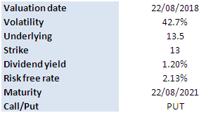
Valuation date:  14 February 2017

Issue date: 1 January 2017

Maturity: 1 January 2019

Coupon: 3%

Credit spread: 0.75%

Risk-free rate: 2%

Stock price: 52

Volatility: 15%

Dividend: 0%

The picture below shows the bond price obtained by using a third-party program.

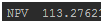
Using the Python program, we obtain a clean price of 113.27

Follow the link below to download the Python program.

Originally Published Here: Valuing a Convertible Bond-Derivative Pricing in Python

How Negative Interest Rates Affect Derivative Pricing Models

As negative interest rates started popping up around the world, quantitative analysts and traders have been asking a mundane but fundamental question: How to price trillions of dollars of financial instruments when their complex pricing models don’t work with negative numbers?

Intuitively, we would say that negative interest rates will affect the prices of interest-rate sensitive instruments such as interest rate swaps and swaptions the most. Indeed, Bloomberg recently elaborated:

The issues are most apparent in the market for interest-rate swaps. (This market allows professional investors to lock in interest rates and lets speculators bet on whether rates on bonds or loans will rise or fall.) That’s because the Black 76 model, the main tool to price options for interest-rate derivatives, and its variants are so-called log-normal forward models. For those who aren’t math nerds, it can essentially be boiled down to this: the formula breaks because it requires users to calculate a logarithm, and a logarithm of a negative number is undefined, or meaningless. Read more

As far as equity derivatives are concerned, the impact will not be as dramatic as with interest-rate sensitive instruments. However, some subtleties in the mathematical approaches can still have an impact on the accuracy of equity-derivative valuation models.

Derivatives traders in equities, on the other hand, have it relatively easy by comparison… sub-zero risk-free rates can cause “approximation errors” for certain kinds of American-style options, which may lead them to become mispriced compared with those used in Europe. Take an American call option on a stock without dividends, for example. Its value will “only equal the European option when the risk-free rate is positive”

Specifically, when we price an American call option, we often argue that if the underlying stock pays no dividend, then it’s never optimal to exercise earlier, i.e. the price of an American call option is equal to its European counterpart.

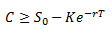
To see this, recall that there exists a lower bound for an American call option on a non-dividend paying stock [1]:

                 where C denotes the price of an American call option

                 S₀ is the stock price

                 K is the strike price

                T  is the time to maturity

                r  is the risk-free interest rate

From this equation, it follows that when r> 0, C >= S₀-K. This means that the American call’s price is always greater than its intrinsic value, therefore it’s never optimal to exercise before maturity.

However, when r<=0, the above condition will no longer be true, and the American call option can be exercised earlier. This will impact the mathematical models that price American options.

 

References

[1] J.C. Hull, Options, Futures, and Other Derivatives, 9^th Edition, 2018

Post Source Here: How Negative Interest Rates Affect Derivative Pricing Models

Are Convertible Bonds Really Attractive?

Investors in South Korea have lost money in a complex derivative linked to constant maturity swap.  In search for higher yields, they are also putting money into another complex financial instrument, convertible bonds. Bloomberg recently reported,

Sales of convertibles, which pay low coupons and let investors convert into stock if the issuer’s shares rise enough, totaled about 3.1 trillion won ($2.5 billion) through July, compared with a record 4.1 trillion won in all of 2018, according to data from Korea Capital Market Institute. Local hedge funds are the main buyers of the bonds, which are usually sold by small- and medium-sized firms without credit ratings. Read more

This convertible bond has a complex feature, and the regulators are worrying that investors will lose money if they don’t fully understand the financial instrument.

Despite near-zero coupon payouts for most of the securities, investors are lured by a “refixing” clause that is unique to Korean convertibles. The term allows a reduction of almost 30% from the initial conversion price if the underlying stock falls.

Regulators are already worried about retail investors owning things they don’t understand. They’re planning a probe into sales of derivative products that carry the risk of losing all their value depending on moves in overseas market rates.

Investing in convertible bonds can add value to a portfolio. However, valuing a convertible bond and managing the risks is not trivial.

A convertible bond (or preferred share) is a hybrid security, part debt and part equity. Its valuation is derived from both the level of interest rates and the price of the underlying equity. Several convertible bond pricing approaches are available to value these complex hybrid securities such as Binomial Tree, Partial Differential Equation and Monte Carlo simulation. One of the earliest approaches was the Binomial Tree model originally developed by Goldman Sachs and this model allows for an efficient implementation with high accuracy. The Binomial Tree model is flexible enough to support the implementation of bespoke exotic features such as redemption and conversion by the issuer, lockout periods, conversion and retraction by the share owner etc.

Originally Published Here: Are Convertible Bonds Really Attractive?

Complex Derivative Linked to Constant Maturity Swap

Yonhap recently reported that South Korea’s investors appear to have lost money by investing in complex derivative products.

The Financial Supervisory Service (FSS) said 3,654 individual investors and 188 businesses were found to have bought 822.4 billion won (US$677.8 million) worth of so-called “derivatives-linked fund” options sold by banks as of Aug. 7.

Such derivative products are structured to track the performance of constant maturity swap, or a swap that allows the purchaser to fix the duration of received flows on a swap, of Treasury bonds of the United States and Britain and the yield of Germany's 10-year state bonds.

The options turned into losers as bond yields in the U.S., Britain and Germany have unexpectedly sank amid speculations that central banks in major economies may aggressively slash their interest rates.

Media reports said some investors bought the options because they were believed to have invested into government bonds of the U.S., Britain and Germany. Read more…

It’s always prudent to invest in what you know. However, in this case, the financial product is probably too complex for the ordinary investors to understand. Its return is linked to the performance of a constant maturity swap.

A constant maturity swap is an interest rate swap where the interest rate on one leg is reset periodically, but with reference to a market swap rate rather than LIBOR. The other leg of the swap is generally LIBOR, but may be a fixed rate or potentially another constant maturity rate. Constant maturity swaps can either be single currency or cross currency swaps. Therefore, the prime factor for a constant maturity swap is the shape of the forward implied yield curves. A single currency constant maturity swap versus LIBOR is similar to a series of differential interest rate fixes (or "DIRF") in the same way that an interest rate swap is similar to a series of forward rate agreements. Valuation of constant maturity swaps depend on volatilities of different forward rates and therefore requires a stochastic yield curve model or some approximated methodology like a convexity adjustment ... Read more...

Originally Published Here: Complex Derivative Linked to Constant Maturity Swap

Stationarity and Autocorrelation Functions of VXX-Time Series Analysis in Python

In the previous post, we presented a system for trading VXX, a volatility Exchange Traded Note. The trading system was built based on simple moving averages.  In this post, we are going to examine the time series properties of VXX in more details.

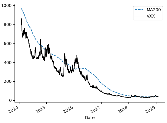
The figure below shows the VXX and its 200-day moving average for the last 5 years. From the Figure, it’s evident that the time series has a strong downward drift. The cause of this downward drift has been discussed to a great extent in the investment community.  It will not be a subject of this post.

Next, we calculate the daily returns of VXX and perform the Augmented Dickey-Fuller test to check the stationarity of the return series.  According to Wikipedia,

..An augmented Dickey-Fuller test (ADF) tests the null hypothesis that a unit root is present in a time series sample. The alternative hypothesis is different depending on which version of the test is used, but is usually stationarity or trend-stationarity. It is an augmented version of the Dickey-Fuller test for a larger and more complicated set of time series models. The augmented Dickey-Fuller (ADF) statistic, used in the test, is a negative number. The more negative it is, the stronger the rejection of the hypothesis that there is a unit root at some level of confidence. Read more

We utilize Python to run ADF test on the return series. The test statistic is -19.5 and the p-value is zero. Therefore the return series is stationary.

We then proceed to examine the autocorrelation functions of VXX returns.

Autocorrelation, also known as serial correlation, is the correlation of a signal with a delayed copy of itself as a function of delay. Informally, it is the similarity between observations as a function of the time lag between them. The analysis of autocorrelation is a mathematical tool for finding repeating patterns... Read more

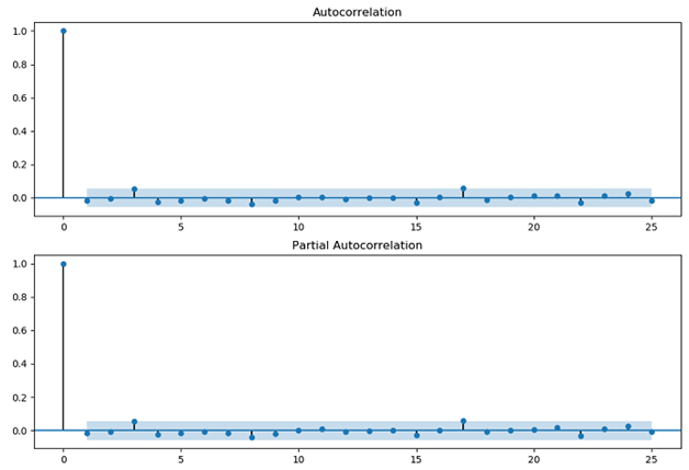
The plot below shows the autocorrelation (ACF) and partial autocorrelation (PACF) functions of VXX returns.

It’s interesting to note that VXX returns are positively auto-correlated at 3-day lag. It’s well-known that the stock indices are mean reverting in the short term. Here we observe the opposite, i.e. a trending property.

Click on the link below to download the Python program and data file.

Post Source Here: Stationarity and Autocorrelation Functions of VXX-Time Series Analysis in Python

A Volatility Trading System-Time Series Analysis in Python

Time series analysis is an important subject in finance. In this post, we are going to apply a time series technique to a financial time series and develop an investment strategy.  Specifically, we are going to use moving averages to trade volatility Exchange Traded Notes (ETN).

Moving averages are used on financial time series data to smooth out short-term noises and identify longer-term trends. We apply them to VXX, a volatility ETN. Note that VXX

• Launched in 2009
• Enables investors to bet on the size of swings in the S&P 500 Index (SPX)
• Used by individual investors and hedge fund managers alike
• Peaked at $2 billion under management in Feb. 2018, now $800 million
• Structured as a debt instrument with a maturity date of Jan. 30, 2019
• Was replaced by the VXXB, which has other features. Read more

The trading rules are as follows [1],

If 10-day Moving Average (MA10) < 30-day Moving Average (MA30) Sell Short

If 10-day Moving Average (MA10) >= 30-day Moving Average (MA30) Cover Short

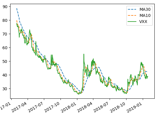
The system is implemented in Python. Graph below shows the MAs and VXX for the last 2 years.

[caption id="attachment_654" align="aligncenter" width="540"] VXX and Moving Averages[/caption]

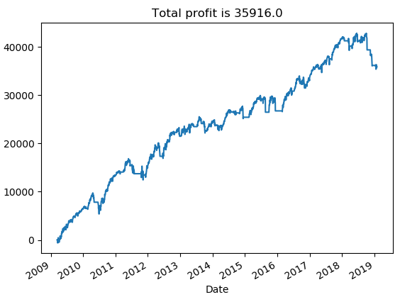
The position size is $10000; leverage is not utilized, and profit is not compounded. Graph below shows the equity curve for the trading strategy from January 2009 to January 2019.

[caption id="attachment_655" align="aligncenter" width="564"] Equity curve for VXX trading system[/caption]

Click on the link below to download the Python program and data file.

 

References

[1] L. Connors, Buy the Fear, Sell the Greed: 7 Behavioral Quant Strategies for Traders, TradingMarkets Publishing, 2018

 

Post Source Here: A Volatility Trading System-Time Series Analysis in Python

Differences Between the VIX Index And At-the-Money Implied Volatility

When trading options, we often use the VIX index as a measure of volatility to help enter and manage positions. This works most of the time. However, there exist some differences between the VIX index and at-the-money implied volatility (ATM IV). In this post, we are going to show such a difference through an example. Specifically, we study the relationship between the implied volatility and forward realized volatility (RV) [1] of SP500. We utilize data from April 2009 to December 2018.

Recall that the VIX index

• Is a model-independent measure of volatility,
• It contains a basket of options, including out-of-the-money options. Therefore it incorporates the skew effect to some degree.

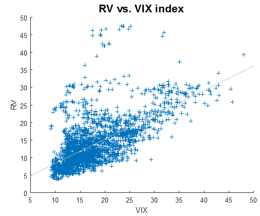
Plot below shows RV as a function of the VIX index.

We observe that a high VIX index will usually lead to a higher realized volatility. The correlation between RV and the VIX is 0.6397.

For traders who manage fixed-strike options, the use of option-specific implied volatilities, in conjunction with the VIX index, should be considered. In this example, we calculate the one-month at-the-money implied volatility using SPY options. Unlike the VIX index, the fixed-strike volatilities are model-dependent. To simplify, we use the Black-Scholes model to determine the fixed-strike, fixed-maturity implied volatilities.  The constant-maturity, floating-strike implied volatilities are then calculated by interpolation.

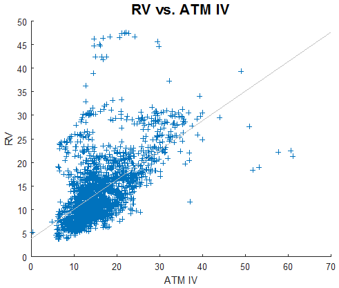
Plot below shows RV as a function of ATM IV.

We observe similar behaviour as in the previous plot. However, the correlation (0.5925) is smaller. This is probably due to the fact that ATM IV does not include the skew.

In summary:

• There are differences between the VIX index and at-the-money implied volatility.
• Higher implied volatilities (as measured by the VIX or ATM IV) will usually lead to higher RV.

Footnotes

[1] In this example, forward realized volatility is historical volatility shifted by one month.

See More Here: Differences Between the VIX Index And At-the-Money Implied Volatility

Valuation of European and American Options-Derivative Pricing in Python

In previous posts, we provided examples of pricing European and American options in Excel. For pricing the European option, we utilized the Black-Scholes formula, and for pricing the American option we utilized the binomial approach. In this post, we are going to implement these methods in Python.

Recall that,

In finance, the binomial options pricing model (BOPM) provides a generalizable numerical method for the valuation of options. The binomial model was first proposed by Cox, Ross and Rubinstein in 1979. Essentially, the model uses a "discrete-time" (lattice based) model of the varying price over time of the underlying financial instrument...

The binomial pricing model traces the evolution of the option's key underlying variables in discrete-time. This is done by means of a binomial lattice (tree), for a number of time steps between the valuation and expiration dates. Each node in the lattice represents a possible price of the underlying at a given point in time.

Valuation is performed iteratively, starting at each of the final nodes (those that may be reached at the time of expiration), and then working backwards through the tree towards the first node (valuation date). The value computed at each stage is the value of the option at that point in time. Read more

We use the same input parameters as in the previous examples.  The main input parameters are as follows,

Figure below shows the results calculated by the Python program. The Python program returns the same values as the Excel workbooks.

Click on the link below to download the Python program.

Originally Published Here: Valuation of European and American Options-Derivative Pricing in Python

Interest Rate Swap-Derivative Pricing in Python

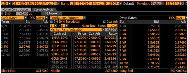
In a previous post, we presented an example of Interest Rate Swap Pricing in Excel. In this post, we are going to provide an example of interest rate swap pricing in Python. We are going to use the USD Libor swap curve as at December 31 2018. Picture below shows the swap curve.

[caption id="attachment_630" align="aligncenter" width="628"] USD Swap Curve as at Dec 31, 2018. Source: Bloomberg[/caption]

Recall that an interest rate swap (IRS) is a financial derivative instrument that involves an exchange of a fixed interest rate for a floating interest rate.  More specifically,

An interest rate swap's (IRS's) effective description is a derivative contract, agreed between two counterparties, which specifies the nature of an exchange of payments benchmarked against an interest rate index. The most common IRS is a fixed for floating swap, whereby one party will make payments to the other based on an initially agreed fixed rate of interest, to receive back payments based on a floating interest rate index. Each of these series of payments is termed a 'leg', so a typical IRS has both a fixed and a floating leg. The floating index is commonly an interbank offered rate (IBOR) of specific tenor in the appropriate currency of the IRS, for example LIBOR in USD, GBP, EURIBOR in EUR or STIBOR in SEK. To completely determine any IRS a number of parameters must be specified for each leg; the notional principal amount (or varying notional schedule), the start and end dates and date scheduling, the fixed rate, the chosen floating interest rate index tenor, and day count conventions for interest calculations. Read more

The valuation of an interest rate swap proceeds as follows,

1. Construction of the zero-coupon curve
2. Determination of the payment schedules
3. Calculation of the net present value of future cash flows

The hypothetical interest rate swap is as follows,

Maturity: 10 years

Notional: 10 Million USD

Fixed rate: 2.5%

Floating rate:  Libor

Note that we utilize the deposit and swap rates only and ignore the futures prices in the bootstrapping process. The values of the fixed, floating legs and the interest rate swap are calculated using a Python program. We obtain the following result

Click on the link below to download the Python program.

Article Source Here: Interest Rate Swap-Derivative Pricing in Python

Weighted Average Cost of Capital (WACC)-Business Valuation Calculator in Excel

In this post, we are going to walk you through an example of calculating the weighted average cost of capital (WACC) using Excel.

The weighted average cost of capital (WACC) is the rate that a company is expected to pay on average to all its security holders to finance its assets. The WACC is commonly referred to as the firm's cost of capital. Importantly, it is dictated by the external market and not by management. The WACC represents the minimum return that a company must earn on an existing asset base to satisfy its creditors, owners, and other providers of capital, or they will invest elsewhere... The WACC is calculated taking into account the relative weights of each component of the capital structure. The more complex the company's capital structure, the more laborious it is to calculate the WACC...Companies can use WACC to see if the investment projects available to them are worthwhile to undertake. Read more

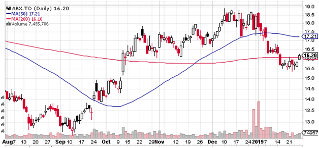
For illustration purposes, we are going to calculate the WACC of Barrick Gold, a major Canadian mining company.

[caption id="attachment_613" align="aligncenter" width="628"] Barrick Gold as at January 25 2019. Source: Stockchart.com[/caption]

The WACC is calculated as follows,

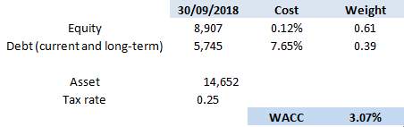
WACC   =E/(E + D)*Cost of Equity + D/(E + D)*Cost of Debt*(1 - Tax Rate)

where E and D denote the market values of the firm’s equity and debt respectively. These numbers are taken from Barrick Q3 financial statement.

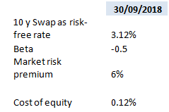
To calculate the cost of equity, we use the Capital Asset Pricing Model (CAPM), according to which the cost of equity is calculated as follows,

Cost of Equity = Risk-Free Rate + Beta * (Market Rate of Return - Risk-Free Rate)

Table below shows the calculation for the cost of equity as at September 30, 2018,

As for the cost of debt, we will use the US Materials B- Yield Curve.  The 10-year yield is 7.651% as at the Q3 financial reporting date.

Finally, we proceed to calculate the WACC. Table below shows the calculation steps and results,

Click on the link below to download the Excel workbook which contains detailed calculation steps and references.

Post Source Here: Weighted Average Cost of Capital (WACC)-Business Valuation Calculator in Excel