Differences Between the VIX Index And At-the-Money Implied Volatility

When trading options, we often use the VIX index as a measure of volatility to help enter and manage positions. This works most of the time. However, there exist some differences between the VIX index and at-the-money implied volatility (ATM IV). In this post, we are going to show such a difference through an example. Specifically, we study the relationship between the implied volatility and forward realized volatility (RV) [1] of SP500. We utilize data from April 2009 to December 2018.

Recall that the VIX index

• Is a model-independent measure of volatility,
• It contains a basket of options, including out-of-the-money options. Therefore it incorporates the skew effect to some degree.

Plot below shows RV as a function of the VIX index.

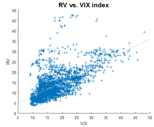
We observe that a high VIX index will usually lead to a higher realized volatility. The correlation between RV and the VIX is 0.6397.

For traders who manage fixed-strike options, the use of option-specific implied volatilities, in conjunction with the VIX index, should be considered. In this example, we calculate the one-month at-the-money implied volatility using SPY options. Unlike the VIX index, the fixed-strike volatilities are model-dependent. To simplify, we use the Black-Scholes model to determine the fixed-strike, fixed-maturity implied volatilities.  The constant-maturity, floating-strike implied volatilities are then calculated by interpolation.

Plot below shows RV as a function of ATM IV.

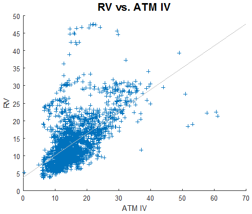
We observe similar behaviour as in the previous plot. However, the correlation (0.5925) is smaller. This is probably due to the fact that ATM IV does not include the skew.

In summary:

• There are differences between the VIX index and at-the-money implied volatility.
• Higher implied volatilities (as measured by the VIX or ATM IV) will usually lead to higher RV.

Footnotes

[1] In this example, forward realized volatility is historical volatility shifted by one month.

See More Here: Differences Between the VIX Index And At-the-Money Implied Volatility

Valuation of European and American Options-Derivative Pricing in Python

In previous posts, we provided examples of pricing European and American options in Excel. For pricing the European option, we utilized the Black-Scholes formula, and for pricing the American option we utilized the binomial approach. In this post, we are going to implement these methods in Python.

Recall that,

In finance, the binomial options pricing model (BOPM) provides a generalizable numerical method for the valuation of options. The binomial model was first proposed by Cox, Ross and Rubinstein in 1979. Essentially, the model uses a "discrete-time" (lattice based) model of the varying price over time of the underlying financial instrument...

The binomial pricing model traces the evolution of the option's key underlying variables in discrete-time. This is done by means of a binomial lattice (tree), for a number of time steps between the valuation and expiration dates. Each node in the lattice represents a possible price of the underlying at a given point in time.

Valuation is performed iteratively, starting at each of the final nodes (those that may be reached at the time of expiration), and then working backwards through the tree towards the first node (valuation date). The value computed at each stage is the value of the option at that point in time. Read more

We use the same input parameters as in the previous examples.  The main input parameters are as follows,

Figure below shows the results calculated by the Python program. The Python program returns the same values as the Excel workbooks.

Click on the link below to download the Python program.

Originally Published Here: Valuation of European and American Options-Derivative Pricing in Python

Interest Rate Swap-Derivative Pricing in Python

In a previous post, we presented an example of Interest Rate Swap Pricing in Excel. In this post, we are going to provide an example of interest rate swap pricing in Python. We are going to use the USD Libor swap curve as at December 31 2018. Picture below shows the swap curve.

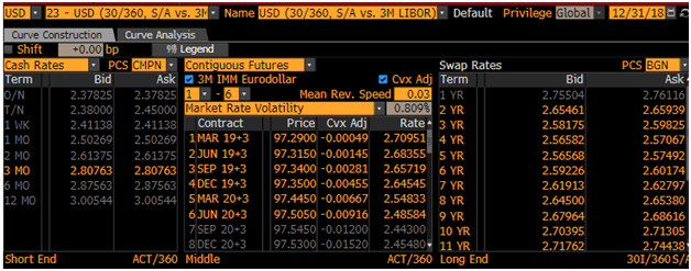
[caption id="attachment_630" align="aligncenter" width="628"] USD Swap Curve as at Dec 31, 2018. Source: Bloomberg[/caption]

Recall that an interest rate swap (IRS) is a financial derivative instrument that involves an exchange of a fixed interest rate for a floating interest rate.  More specifically,

An interest rate swap's (IRS's) effective description is a derivative contract, agreed between two counterparties, which specifies the nature of an exchange of payments benchmarked against an interest rate index. The most common IRS is a fixed for floating swap, whereby one party will make payments to the other based on an initially agreed fixed rate of interest, to receive back payments based on a floating interest rate index. Each of these series of payments is termed a 'leg', so a typical IRS has both a fixed and a floating leg. The floating index is commonly an interbank offered rate (IBOR) of specific tenor in the appropriate currency of the IRS, for example LIBOR in USD, GBP, EURIBOR in EUR or STIBOR in SEK. To completely determine any IRS a number of parameters must be specified for each leg; the notional principal amount (or varying notional schedule), the start and end dates and date scheduling, the fixed rate, the chosen floating interest rate index tenor, and day count conventions for interest calculations. Read more

The valuation of an interest rate swap proceeds as follows,

1. Construction of the zero-coupon curve
2. Determination of the payment schedules
3. Calculation of the net present value of future cash flows

The hypothetical interest rate swap is as follows,

Maturity: 10 years

Notional: 10 Million USD

Fixed rate: 2.5%

Floating rate:  Libor

Note that we utilize the deposit and swap rates only and ignore the futures prices in the bootstrapping process. The values of the fixed, floating legs and the interest rate swap are calculated using a Python program. We obtain the following result

Click on the link below to download the Python program.

Article Source Here: Interest Rate Swap-Derivative Pricing in Python