Saturday, August 29, 2020

Valuation of Callable Puttable Bonds-Derivative Pricing in Python

In a previous post, we presented a method for pricing a fixed-rate bond. In this post, we are going to discuss valuation of a callable bond.

A callable bond (also called redeemable bond) is a type of bond (debt security) that allows the issuer of the bond to retain the privilege of redeeming the bond at some point before the bond reaches its date of maturity. In other words, on the call date(s), the issuer has the right, but not the obligation, to buy back the bonds from the bond holders at a defined call price. Technically speaking, the bonds are not really bought and held by the issuer but are instead cancelled immediately.

The call price will usually exceed the par or issue price. In certain cases, mainly in the high-yield debt market, there can be a substantial call premium.

Thus, the issuer has an option which it pays for by offering a higher coupon rate. If interest rates in the market have gone down by the time of the call date, the issuer will be able to refinance its debt at a cheaper level and so will be incentivized to call the bonds it originally issued. Another way to look at this interplay is that, as interest rates go down, the present values of the bonds go up; therefore, it is advantageous to buy the bonds back at par value. Read more

Valuation of a callable bond requires a short-rate model. The valuation steps are as follows,

  1. Calibrate the short-rate model using market data
  2. Build an interest-rate tree
  3. Price the bond

[caption id="attachment_991" align="aligncenter" width="520"]valuation of callable bond Swaption volatilities. Source: Bloomberg[/caption]

We are going to present a concrete example of pricing a callable bond. The parameters of a hypothetical callable bond are as follows,

Valuation date: June 30, 2020

Issue date: September 30, 2019

Maturity: 5 years

Coupon: 2.5%

Call strike: 100

Call period: September 30, 2019 to maturity

We chose the Hull-White model to describe the interest rate dynamics.  This model is widely used in practice because it allows for the model to fit the term structure of interest rates. We utilize the method presented in Reference 1 in order to calibrate the model parameters to the market data. Specifically, we use swaption volatilities in the calibration and obtain σ=0.676% and α=0.127% as at the valuation date.

We then use a Python program to build a trinomial tree for the risk-free rates following the procedure detailed in References 2 and 3. After a trinomial interest-rate tree is built, the valuation of the callable bond proceeds as follows.

Let’s define the following terms with respect to a node (i,j) :

  • i: means that on the node (i,∙) the date is defined by i×dt where dt is the length of the time-step.
  • j: means the position (up/medium/down) of the tree,
  • C (i,j): call price at node (i,j),
  • P (i,j): put price at node (i,j) ,
  • R (i,j): the projected risk-free rates at nodes (i,j) which are modeled using the Hull-White interest rate dynamics,
  • V(i,j): continuation value of the bond at node (i,j) which is calculated as the expectation value of the continuation values of the next three possible nodes originating from (i,j) discounted by one period using the projected rates R(i,j).

The values of the bond at the terminal nodes N, where N=T/dt, and T is the time to maturity, is set to the notional at maturity (Notional_N) plus the interest payment at that time (interest_N), i.e.

V(N,∙)=Notional_N+ interest_N,

We then move back to the previous time step and calculate the bond continuation value at each node on this time slice using the continuation values at its precedent nodes and add any interest payment that occurs between the two time steps.

If the bond is callable at time i×dt, then the value of the bond is calculated as,

V(i,j)=min( V(i,j),C(i,j))

i.e. the issuer will exercise the call if the call value is smaller than the continuation value; that is, the position of the issuer can be improved by calling the bond.

Similarly, if the bond is puttable at time i×dt, then the value of the bond is calculated as,

V(i,j)=max( V(i,j),P(i,j))

i.e. the bond holder will exercise the put if the put value is greater than the continuation value.

The above procedure is repeated until we reach the root of the tree. The value of the callable/puttable bond at the valuation date is the continuation value at time zero.

The picture below shows the price of the hypothetical callable bond calculated by the Python program.

pricing a callable bond

Click on the link below to download the Python program.

References

[1] Hull, J. C. (2018), Options, Futures and Other Derivatives (10th Ed.), Prentice-Hall

[2]  Hull, J. C. and White, A. 1994, Numerical Procedures for Implementing Term Structure Models I: Single Factor Models, Journal of Derivatives

[3]  Hull, J. C. and White, A. 1996, Using Hull-White Interest-Rate Trees, Journal of Derivatives

Post Source Here: Valuation of Callable Puttable Bonds-Derivative Pricing in Python

Thursday, August 27, 2020

Short Volatility Funds Lost Money During The Pandemic

With a sudden increase in volatility during the pandemic, many volatility funds lost money.

Many funds were struck because they adopted a strategy known as shorting volatility — betting that it will fall or remain low. Such funds sell derivative protection such as put options, which give the buyer the right to sell at a pre-determined price. They earn money by effectively writing market insurance, hoping that volatility — which helps determine options prices — will remain low and the options will expire worthless.

volatility hedge fund

Many investors have been lured into taking this approach over the past decade by years of gently rising markets and mild market moves, fuelled by trillions of dollars of central bank stimulus, which have helped such funds make money. Read more

One of the most notable cases was the Alberta Investment Management Corporation’s loss of $3 billion.

The Alberta Investment Management Corp. — which manages pension assets, sovereign wealth, and other public money — lost billions of dollars on wrong-way volatility trades when markets crashed earlier this year, and then shut down the strategies, according to informed sources.

The now-defunct volatility-trading program cost pensioners and Albertans about $3 billion, the sources said. That’s on top of substantial, first-quarter losses to portfolio value that nearly all public funds are dealing with amid the coronavirus crisis. Read more


Originally Published Here: Short Volatility Funds Lost Money During The Pandemic

Tuesday, August 25, 2020

Banks Hold Many Illiquid Assets

The trend in the increased holding of risky assets continues. Because of Covid-19, the big banks now hold more illiquid, opaque assets than before.

Lenders including Barclays Plc, Citigroup Inc., BNP Paribas SA and Societe Generale SA reported a surge of more than 20% in their most opaque assets during the chaotic first half of 2020, Bloomberg calculations show. The banks are now sitting on hard-to-value trades that they say are worth about $250 billion, including categories that gained notoriety during the financial crisis, such as complex debt securities.

illiquid assets

These assets are hard to value, and they can cause a financial crisis like the one we had in 2008.

There’s little market data for Level 3 assets -- which include distressed debt, some mortgage-backed bonds, high-risk loans and derivatives linked to everything from interest rates to corporate debt -- so banks get to value them based on historical trends and their own risk assumptions. Read more

Originally Published Here: Banks Hold Many Illiquid Assets

Monday, August 24, 2020

Quantitative Trading

If you’re looking to set up your own algorithmic trading business, quantitative trading is a market you can consider. Many independent investors are exploring the market, learning to generate data, and execute it.

In the past, quantitative trading used to be the business of hedge funds and other financial institutions involving huge sales of shares. The shares in this business run in many hundred thousands, together with the securities. Working for a hedge fund may be the reason you learn about the quantitative trading system.

What is quantitative trading?

Quantitative trading involves using quantitative analysis to identify points with a profitable trade where you can buy assets. This is a branch of quantitative finance. To find an opportunity for trading, a trader has to compute a set of mathematical data in order to determine a market is most likely profitably within a period.

The type of asset involved in a single quantitative trade and the type of research used in the analysis will be the trader’s sole choice. The process of developing a workable trading strategy requires careful study and testing to ascertain the loops in the system before the execution.

Heavy mathematical modeling and computation form the basis of quantitative analysis trading. To keep up with these computations, a trader has to be versed in a relevant computer program. Some of these programs include MATLAB, Python, R, C/C++, network latency optimization, etc.

quantitative trading

Breakdown of Quantitative Trading

In quantitative trading, your business is to use the mathematical models you generate to learn the possibility of getting a certain outcome. The only possible way to achieve this in quantitative finance is by using programming and statistics. Your interest is in the volume and price of a trade, not in the strength of the brand.

Therefore, assume that the stock of a certain business rises in volume, which also affects its pricing. You then work out a program targeted at identifying how this pattern occurs in the history of the business. How does this kind of rise affect the market value of this business?

Let’s say the result of your research says the business has experienced a 90% growth from this type of rise over the years. It means that there's a 90% chance for such growth in the future.

Who does Quantitative Trading?

People who have a background in financial modeling, math, or engineering are more likely to excel in quantitative analysis, and by extension, quantitative trading. Added to these skills, these individuals need a strong understanding and ability to handle any of the programming software that includes Python, R, and C/C++, plus APIs (application programming interfaces).

Some of the added skills that a funds company will need a person to have included being able to create automated data and mine data. These are the same skills an individual trader needs. However, you should also have a proficiency in understanding kurtosis, VaR (Value at Risk), and conditional probability.

Quantitative trading involves mathematical computations in all of its entirety. This feature is what distinguishes it from the traditional investment platform where you consider brand behavior.

A trait that you’ll find among traders is that they may decide to customize an existing strategy that is proven as successful, in addition to building their own. They go ahead to create programs that help them identify the opportunities in a strategy, thereby creating time to research more strategies.

A part of the job of quantitative traders is the high-frequency trading (HFT). In HFT, they work on many positions in the short term, opening and closing with the help of programming.

This strategy is not for every fund group or trader. In some cases, the trader uses a model to find out trades that are larger and less frequent as part of their strategy for the long-term.

Traders who use HFT need computer programs for this technique because it involves so many short transactions that should be identified and executed at once. A programming strategy would be more efficient than human analysis to avoid time lapse and loss.

Major components of Quantitative Trading

Singling out opportunities and executing them are the basics of every quantitative trading system. Every system is unique in the way it identifies positions and executes. But, the components are integrated across the board.

They include:

  • Identifying the Strategy
  • Backtesting it
  • System of Execution
  • Risk Management

Here’s a breakdown of these concepts.

Identifying the Strategy

Every process of quantitative trading starts with research. Research helps you to find your strategy. You can analyze this strategy by fitting it into your existing portfolio, to check if it aligns with your other strategies. Further, obtain all data necessary to test your strategy while optimizing it for lower risks and more returns.

As an individual trader, factor in the costs involved, including your capital and the effect of these transactions.

Public sources can be a good place to find strategies that are profitable. These sources include trade journals, academic publications, and quantitative finance blogs. The details they offer vary as well.

Public source strategies do not include the parameters and methods of tuning. If you are able to find a suitable pattern for optimizing them, these can become highly profitable strategies.

A strategy can have Low-frequency trading (LFT), high-frequency trading HFT), and Ultra-high frequency trading (UHFT). These frequencies refer to how long a strategy will hold an asset. LFT will stay longer than one trading day; HFT will hold intraday and UHFT will hold for milliseconds and seconds.

With your strategy set up, the next thing is to backtest it, to know how profitable it is.

Backtesting your strategy

In backtesting, you apply the strategy you picked to both historical and out-of-sample data to prove that it is profitable. Your result tells you what to expect of the strategy in a real trade, even though it doesn’t always translate exactly.

While backtesting, you’ll meet several biases; you’ll need to consider them diligently before eliminating them. The biases will include look-ahead bias, data-snooping bias, and survivorship bias.

Also, look out for how clean and available historical data is, which includes providing a backtesting platform that is robust and costs that are realistic.

After identifying a strategy, get the historical data since this will help you with testing and refinement. Here are some issues that concern using a historical set of data.

Cleanliness/Accuracy

Does the data contain any error? In some cases, it’s easy to pick out errors. Other times, it’s well-hidden in plain sight. If possible, have a team of providers who weigh their data with each other to identify biases.

Survivorship bias

Does the data contain delisted or bankrupt stocks? Are the assets still trading?

Survivorship bias is a feature you look out for in a cheap set of data. You want to know if the assets are in a trade or not. Trades that have left the market or bankrupt stocks will not perform in real life.

Besides, cheap data will often perform better during backtesting than they would in the real world.

Corporate actions

What are the dividend adjustments and stock splits in the trade? That is, activities of the company that take away from the price returns.

In all cases, movements will create a step-function change in the raw price of the company. This change does not form part of the price returns when you’re calculating. In fact, you should carry out back adjustments when you make these changes. You want to avoid confusing a stock split with actual returns adjustments.

When you’ve established your history data set, you need a software platform that can be either of a dedicated backtest software, a complete custom implementation using a programming language, or a numerical platform.

To measure the performance of your strategies, you’ll need to know the maximum drawdown and the Sharpe Ratio. In maximum drawdown, you’re measuring the equity curve drop from peak to trough in a specific period, as a percentage.

In Sharpe Ratio, you’re taking the average of the excess returns and dividing it by their standard deviation. This excess return is measured against the expected benchmark for the strategy’s return.

Done with backtesting, you can then execute.

System of Execution

With the list of trades your strategy has generated, you can build a manual execution system or an automated system. In a manual system, your business is to keep your broker on a call while you place your trades. Otherwise, build a semi-automated or fully-automated system for your execution.

An LFT strategy will thrive on manual or semi-automated systems while HFT strategies are best suited for fully-automated systems. Automated systems help you create extra time to look for more strategies and run them.

3 factors you should consider in creating your execution system include your broker’s interface, how to minimize transaction costs and performance divergence from backtested performance.

Individual traders will often handle their execution themselves while established hedge funds will have their dedicated executor.

In executing, you also need to minimize the cost of transactions which includes commissions, slippage, and spread. The brokerage charges commissions; slippage tells the difference in the price of your order and your initial estimate, while the spread is the gap in the bid/ask price of the security you’re trading. Spread, however, is not a constant factor.

Transaction costs, in itself, can be the shift from a very unprofitable strategy to a highly profitable strategy. These costs can barely be detected in a backtest, which is why you need to be critical about analyzing your transaction costs.

About divergence of strategy from backtested performance, some bugs and invisible trading strategies may only emerge in life transactions. Some of them include a new regulatory environment, macroeconomic phenomena, and change in investor sentiment. All these are in addition to life-ahead, data snooping, and survivorship biases.

Risk Management

Risk management includes your ability to work around the list of biases mentioned before. It also includes the risk of technology (like a dysfunctional server) and brokerage bankruptcy. Think of anything that can impact the trading system; it’s a risk you should manage.

Portfolio theory (i.e. optimal capital allocation) is part of the risk management system. It’s about deciding how to allocate funds to the various strategies and the trades that lie within each strategy. It’s a complex system that requires great thought and diligent execution.

Your personal disposition could also be a threat to your trades. It’ll determine how fast you are with making decisions, your ability to dispassionately make a good decision and to cancel out the greed in your trades.

Pros and Cons of Quantitative Trading

The pros and cons associated with this business is embedded in the transactional process and the returns from it. They are as follows:

Pros

  • Quantitative Trading helps you determine how profitable a system before executing a trade
  • You can arrive at a less flawed decision through monitoring and analysis before the system is overwhelmed with data
  • Computers are efficient in automated monitoring and analysis, therefore enhancing the rate of decision making
  • Access to a large market and extensive data points list
  • Less emotional involvement since AI handles a good part of the decision making system

Cons

  • Ability to remain as dynamic as the financial market system.
  • Strategies are often momentarily profitable. Many do not survive changes in the market condition

Conclusion

Quantitative trading is a model that uses mathematical computation to determine existing opportunities. This requires quantitative traders to have an extensive background in mathematics, statistics, programming, and related fields. Creating an effective quantitative trading system requires 4 components including strategy, backtesting, execution, and risk management.

A good majority of quantitative traders work for established systems such as investment firms and hedge funds. However, individuals are beginning to start their own quantitative trading and require more computational skills since they have to manage the system alone.


Quantitative Volatility Trading

In this part, we will look at volatility trading from the quantitative perspective.

We first need to estimate the current volatility

Close-to-Close Historical Volatility

The Close-to-Close Historical Volatility has the following characteristics [1]

Advantages

  • It has well-understood sampling properties
  • It is easy to correct bias
  • It is easy to convert to a form involving typical daily moves

Disadvantages

  • It is a very inefficient use of data and converges very slowly

Parkinson Historical Volatility

The Parkinson volatility has the following characteristics

Advantages

  • Using daily ranges seems sensible and provides completely separate information from using time-based sampling such as closing prices

Disadvantages

  • It is really only appropriate for measuring the volatility of a GBM process. It cannot handle trends and jumps
  • It systematically underestimates volatility.

Garman-Klass Historical Volatility

The Garman-Klass volatility estimator has the following characteristics

Advantages

  • It is up to eight times more efficient than the close-to-close estimator
  • It makes the best use of the commonly available price information

Disadvantages

  • It is even more biased than the Parkinson estimator

Garman-Klass-Yang-Zhang Historical Volatility

We note that the Garman-Klass-Yang-Zhang  volatility estimator takes into account overnight jumps but not the trend, i.e. it assumes that the underlying asset follows a GBM process with zero drift. Therefore the GKYZ volatility estimator tends to overestimate the volatility when the drift is different from zero. However, for a GBM process, this estimator is eight times more efficient than the close-to-close volatility estimator.

We now present a volatility trading system on a volatility ETF.

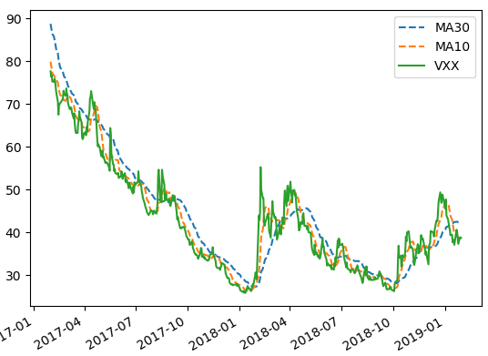
The trading rules are as follows

If 10-day Moving Average (MA10) < 30-day Moving Average (MA30) Sell Short

If 10-day Moving Average (MA10) >= 30-day Moving Average (MA30) Cover Short

The system is implemented in Python. Graph above shows the MAs and VXX for the last 2 years

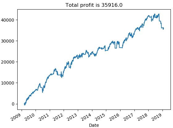
The position size is $10000; leverage is not utilized, and profit is not compounded. Graph below shows the equity curve for the trading strategy from January 2009 to January 2019.

quantitative volatility trading

References

[1]  E. Sinclair, Volatility Trading, John Wiley & Sons, 2008


Article Source Here: Quantitative Trading
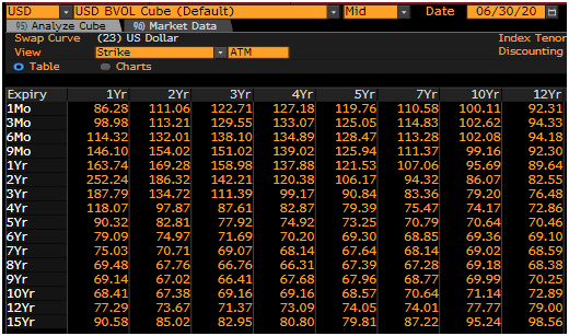
Saturday, August 22, 2020

Convertible Bond Issuance Has Increased

Convertible bond issuance has increased during the Covid 19 pandemic.

From a funding perspective, convertible bonds have many attractive features for corporates, which have become more important during the pandemic.

...In volatile markets, the value of the embedded option in a convertible bond increases. The asset class also becomes more attractive to investors owing to its convexity. Convertible bonds give investors equity-like returns on the upside while maintaining bond-like protections on the downside. Read more

What is a convertible bond?

... a convertible bond or convertible note or convertible debt (or a convertible debenture if it has a maturity of greater than 10 years) is a type of bond that the holder can convert into a specified number of shares of common stock in the issuing company or cash of equal value. It is a hybrid security with debt- and equity-like features. It originated in the mid-19th century, and was used by early speculators such as Jacob Little and Daniel Drew to counter market cornering. Read more

Despite their attractive features, when investing in convertible bonds, investors should pay particular attention to the credit risks of the issuers and the sector in general.

A bigger concern, and one that will hold the market back, is credit quality. The convertible bond market is now even more highly exposed to the technology sector, where companies often lack positive free cash flow. Any bursting of the bubble in tech stocks will be disastrous for the performance of convertible bonds.

Accurate pricing and risk management of convertible bonds are vital for the success of investing in convertible bonds.

Post Source Here: Convertible Bond Issuance Has Increased

Thursday, August 20, 2020

How to Forecast Implied Volatility

How do you determine the volatility of an unlisted entity, and more generally, how do you forecast volatility? These are non-trivial questions. There is an interesting discussion on Stackexchange:

Here is a question I had for a long time but I never asked. Let's take an easy example, AirBnb will likely have an IPO soon, the stock will be quoted on the market. Let's say I would like to price an option on this stock, how would I proceed?

For sure I could sell some with a premium equal to the spot, and wait for the secondary market to adjust, and then extract the IV to do a better pricing, but I would still need to find people to buy at that price.

So in practice how does it work, there is no underlying historical data, nor implied volatility available. Read more

The following could be a solution

With completely no historical stock price, the best I can think of is to find several companies in the same business (e.g. BOOKING for AIRBNB) and look at the range of their vols. Then estimate which percentile it will be in this range according to the size of the company. This is very very raw estimate. Once the stock starts trading then you can adjust.

More discussion on volatility trading can be found in Colin Bennett’s book Trading Volatility: Trading Volatility, Correlation, Term Structure and Skew

Post Source Here: How to Forecast Implied Volatility

Tuesday, August 18, 2020

Valuation of Warrants-Derivative Pricing in Python

A warrant is a financial derivative instrument that is similar to a regular stock option except that when it is exercised, the company will issue more stocks and sell them to the warrant holder.

Warrants and options are similar in that the two contractual financial instruments allow the holder special rights to buy securities. Both are discretionary and have expiration dates. The word warrant simply means to "endow with the right", which is only slightly different from the meaning of option.

Warrants are frequently attached to bonds or preferred stock as a sweetener, allowing the issuer to pay lower interest rates or dividends. They can be used to enhance the yield of the bond and make them more attractive to potential buyers. Warrants can also be used in private equity deals. Frequently, these warrants are detachable and can be sold independently of the bond or stock.

...Warrants issued by the company itself are dilutive. When the warrant issued by the company is exercised, the company issues new shares of stock, so the number of outstanding shares increases. When a call option is exercised, the owner of the call option receives an existing share from an assigned call writer (except in the case of employee stock options, where new shares are created and issued by the company upon exercise). Unlike common stock shares outstanding, warrants do not have voting rights. Read more

The valuation of warrants is similar to the valuation of stock options except that the effect of dilution should be considered. In this post, we first look at the valuation of warrants without the dilution effect. After that, we will discuss the valuation model that takes dilution into account.

The valuation model will be based on Cox, Ross, and Rubinstein (CRR) binomial tree [1]. In 1979, Cox, Ross and Rubinstein proposed a numerical method for pricing American style options using a binomial tree. This is a tree that represents possible paths that might be followed by the underlying asset’s price over the life of the warrant. The model works by dividing the time to expiration into several time intervals. Over each time interval, the model assumes that the price of the underlying asset moves up or down to certain values. The magnitude of these moves is determined by the volatility of the underlying asset and the length of the time step. The time slices and the simulated prices of the underlying asset at these times form the nodes of the binomial tree.

After a binomial tree is built, the valuation of the warrant proceeds as follows,

  1. Calculate the warrant value at each end node of the tree.
  2. Move on to the previous time step and calculate the warrant value at each node on this time slice using the warrant values at the precedent nodes.
  3. After the warrant value is calculated at a node, check whether early exercise is allowed and optimal. The warrant price at this node is then the greater of this value and the payoff of the early exercise.
  4. Continue in this manner until the warrant is valued at all nodes of the tree.
  5. The value at the root node of the tree is the price of the warrant at the valuation date.

We now discuss the dilution effect. If the issuance of warrants was announced publicly, then under the Efficient Market Hypothesis, it is reasonable to assume that the stock price after the announcement already reflects the dilution. In this case, the dilution effect can be ignored in the valuation model.  If, on the other hand, the issuance of warrants was not announced publicly, which is often the case of private companies, then dilution should be taken into account explicitly.

The dilution effect can be accounted for by recalculating the share price at each node (i, j) of the tree as follows,

valuation of warrants with dilution

where and represent the indices of time and stock positions in the tree, respectively,

           N is the number of warrants and,

          K is the strike price.

We implemented the above valuation method in Python.  The input parameters are as follows,

Stock price: 50

Strike: 50

Maturity: 5 years

Risk-free rate: 2%

Volatility: 40%

Number of outstanding shares: 1,000,000

Number of warrants: 50,000

The picture below shows the warrant prices with and without the dilution effect.

valuation of warrants

Follow the link below to download the Python program.

References

[1] Cox, J. C.; Ross, S. A.; Rubinstein, M. (1979). Option pricing: A simplified approach. Journal of Financial Economics. 7 (3): 229.

Post Source Here: Valuation of Warrants-Derivative Pricing in Python

Monday, August 17, 2020

Impact of a Low Correlation Trading Strategy

When constructing a portfolio, adding a low correlation, low Sharpe ratio strategy can have the same impact as adding a high Sharp ratio strategy. The low correlation strategy is a great diversifier.

The core argument presented in this paper –that SR is a misleading index of whom a fund should hire or fire– seems at odds with standard business practices. The SR Indifference Curve shows that even PMs with a negative individual SR should be hired if they contribute enough diversification. Why is that not the case? Because of a netting problem: A typical business agreement is that PMs are entitled to a percentage of their individual performance, not a percentage of the fund’s performance. Legal clauses may release the fund from having to pay a profitable PM if the overall fund has lost money, however that PM is unlikely to remain at the firm after a number of such events. This is a very unsatisfactory situation, for a number of reasons: First, funds are giving up the extra-performance predicted by the SR Indifference Curve. Second, funds are compelled to hire ‘star-PMs’, who may require a high portion of the performance fee. Third, funds are always under threat of losing to competitors their ‘star-PMs’, who may leave the firm with their trade secrets for a slightly better deal. In some firms, PMs’ turnover is extremely high, with an average tenure of only one or two years. Read more

Article Source Here: Impact of a Low Correlation Trading Strategy

Saturday, August 15, 2020

Accounting in Quantitative Finance

Is knowledge of accounting important in the field of quantitative finance?  A poster believes that it is important:

Accounting is a vital skill if you end up in a managerial position, and unless your career goal is to always be a cog in someone else's clockwork, then you will eventually find yourself in a managerial/senior partnership position even through quant research. I still play a critical role in my firm's quant strategies team, but here's a few things I've had to do that relate to accounting that you'd find common on the buy-side:

    Fighting those inconsistencies in our PBs/clearing firms' trade execution reports.

    Negotiating fund administrators' fee structures and services and interfacing their platform(s) with our internal tools.

    Voting on the decision whether to take incentive fees or allocations.

    Voting on the decision on 475(f) election (at a multi-asset class hedge fund, where the proportion of short-term gain isn't immediately clear and knowledge of individual strategies' PnL was important in making this decision).

    Defending a cap table and business valuation (merger of two prop firms).

    Voting on a decision whether to restructure our fund management company as an LP (this was intricately tied to our partners' bonuses, because of changes to NII and SE tax policy arising from the Affordable Care Act).

Now, purely on the quant research and strategy development end, accounting is an extremely useful skill for obtaining and scrubbing your primary data source for trading decisions:

    Price-moving information, e.g. book value, debt/equity ratio, operating income to interest expenses, could be contained in unstructured accounting statements.

    Trading opportunities could arise from discrepancies due to reporting practices, e.g. mark-to-market, mark-to-close etc.

    Trading opportunities could arise from accounting inconsistencies, e.g. miscategorization.

    Market price of assets may be overestimated/underestimated significantly if they are based on expected future cash flows.

    Valuation based on discounted cash flow.

Read more


While other reader believes that it’s not important.

A quant may find accounting useful occasionally but it is really tangential knowledge. I would not consider typical financial or managerial accounting as pre requisites for a Quant Fin program.

That said, certain quants in fixed income or credit do end up dealing with intricacy of cash flows. Accounting background will help in those scenarios.


So what do you think? Let us know

Article Source Here: Accounting in Quantitative Finance

Wednesday, August 5, 2020

Performance Share Units-Derivative Valuation in Python

In a previous post, we wrote about Employee Stock Options, a form of financial compensation that a company uses to reward its employees. In this post, we are going to discuss another form of compensation, Performance Share Units.

Performance share units (PSUs) are hypothetical share units that are granted to you based mainly on corporate and/or individual performance. Structurally, they are very similar to restricted stock units except these are more focused on your performance. These notional units fluctuate in value based on the underlying company stock but do not represent actual share ownership until you convert them to shares. They are designed to mirror share ownership and you will generally be granted additional units having the same value as dividends being paid on the regular shares.

Companies typically use PSUs as a form of mid-term compensation as the units usually vest after three years. It converts an amount that would normally be paid as a bonus or other cash remuneration to share ownership. It is meant to encourage employees to meet certain performance targets and maximize share value over the medium-term. If the performance target is not met, the shares the employees could have received are forfeited to the company [1].

The valuation of PSUs is based on the same principles similar to the valuation of stock options.  However, more often than not, the payoff of a PSU is more complex and is usually tied to a relative performance measure. Therefore, Monte Carlo simulation is a preferred choice for pricing PSUs.

To price a PSU, we first simulate the price paths using the following Stochastic Differential Equation:

Performance Share Units

where

  • St is the stock price at time t,
  • σ denotes the stock volatility,
  • µ is the drift which equals the risk-free rate, and
  • dWt represents the standard normal random variable.

The simulation is carried out until the PSU’s maturity. We then implement the payoff function and calculate the mean value of the payoff. Finally, we discount the mean value to the present and obtain the PSU value.

The Monte Carlo program used for pricing stock options can be modified without difficulty to implement the particular payoff of a PSU. If a relative performance with respect to an index or other stocks is required, then we need to perform Monte Carlo simulations involving multiple assets [2].

Follow the link below to download the Python program for performing Monte Carlo simulations.


References

[1] The Navigator, RBC Wealth Management,  June 2018

[2] Glasserman, Paul; Monte Carlo Methods in Financial Engineering, Springer; 2003


Post Source Here: Performance Share Units-Derivative Valuation in Python