What is Stock Beta and How to Calculate Stock Beta in Python

In finance, beta measures a stock's volatility with respect to the overall market. It is used in many areas of financial analysis and investment, for example in the calculation of the Weighted Average Cost of Capital, in the Capital Asset Pricing Model and market-neutral trading.

Beta of an investment is a measure of the risk arising from exposure to general market movements as opposed to idiosyncratic factors.

The market portfolio of all investable assets has a beta of exactly 1. A beta below 1 can indicate either an investment with lower volatility than the market, or a volatile investment whose price movements are not highly correlated with the market. An example of the first is a treasury bill: the price does not fluctuate significantly, so it has a low beta. An example of the second is gold. The price of gold fluctuates significantly, but not in the same direction or at the same time as the market.

A beta greater than 1 generally means that the asset both is volatile and tends to move up and down with the market. An example is a stock in a big technology company. Negative betas are possible for investments that tend to go down when the market goes up, and vice versa. There are few fundamental investments with consistent and significant negative betas, but some derivatives like put options can have large negative betas. Read more

In this post, we present a concrete example of calculating the beta of Facebook, a technology stock. As for the market benchmark, we utilize SPY.

The beta of a financial instrument is calculated as follows,

where

• r_S is the stock return,
• r_M is the market return,
• Cov denotes the return covariance and,
• Var denotes the return variance.

We downloaded 5 years of data from Yahoo Finance and implemented equation (1) in Python.  The picture below shows the result returned by the Python program

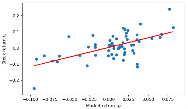
It’s observed that the beta of Facebook is 1.19, which means that Facebook is more volatile than the market.

The next picture shows the stock returns regressed against market returns. Note that the slope of the linear regression line equals the beta of the stock.

Follow the link below to download the Python program.

Article Source Here: What is Stock Beta and How to Calculate Stock Beta in Python

Correlation Between the VVIX and VIX indices

The VIX index is an important market indicator that everyone is watching. VVIX, on the other hand, receives less attention. In this post, we are going to take a look at the relationship between the VIX and VVIX indices.

While the VIX index measures the volatility risks, VVIX measures the volatility-of-volatility risks. Its calculation methodology is similar to the VIX’s except that instead of using SPX options it uses VIX options.

To study the relationship between these 2 indices, we first calculated the rolling 20-days correlation of the VIX and VVIX returns from January 2007 to March 2020. The median value of correlation is 0.807 and 25% quantile is 0.66

The figure below presents the rolling 20-days VIX/VVIX correlation for the last 2 years. We also superimposed SPY on the chart. We observe that the correlation is usually high but there are periods where it decreases significantly. The current period is one of those.

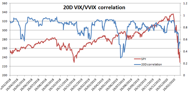
[caption id="attachment_393" align="alignnone" width="628"] Correlation between the VVIX and VIX indices[/caption]

The next figure shows the scatter plot of VVIX returns vs. VIX returns. It’s observed that there is a significant population where VIX and VVIX returns are of opposite signs.  We subsequently calculated the number of instances where VIX and VVIX move in the opposite direction. This indeed happens 22% of the time.

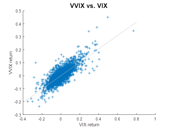
[caption id="attachment_394" align="aligncenter" width="563"] VVIX returns vs. VIX returns[/caption]

Some implications of this study are:

• Although the correlation between VIX and VVIX appears to be high, there is a significant number of instances where VIX and VVIX move in the opposite direction. So it’s fair to say that VVIX follows separate price dynamics which is different from the VIX. In other words, VVIX prices in different risks.
• Long VIX options or SPX back spreads are not always a good hedge for an equity portfolio. The hedge can break down.
• At times it’s cheaper to hedge a long equity portfolio using SPX options; at times it’s cheaper using VIX options.

See More Here: Correlation Between the VVIX and VIX indices

Value At Risk – Financial Risk Management in Python

Value at Risk (VaR) is a tool for measuring a portfolio’s risk.

Value at risk (VaR) is a measure of the risk of loss for investments. It estimates how much a set of investments might lose (with a given probability), given normal market conditions, in a set time period such as a day. ... For a given portfolio, time horizon, and probability p, the p VaR can be defined informally as the maximum possible loss during that time after we exclude all worse outcomes whose combined probability is at most p. This assumes mark-to-market pricing, and no trading in the portfolio.

For example, if a portfolio of stocks has a one-day 5% VaR of $1 million, that means that there is a 0.05 probability that the portfolio will fall in value by more than $1 million over a one-day period if there is no trading. Informally, a loss of $1 million or more on this portfolio is expected on 1 day out of 20 days (because of 5% probability). Read more

There are basically 3 methods for calculating the VaR [1]

1. Historical simulation
2. Variance-covariance approach
3. Monte Carlo simulation

In this post, we implement the 3^rd method, i.e. the Monte Carlo simulation, in Python.  More details of the methodology can be found in Ref [1].

The simulation parameters are as follows,

• Portfolio value: $1 Million
• Confidence interval: 95%
• Time horizon: 1 day
• Underlying: SPY

We utilize 5-years daily data of SPY retrieved from Yahoo Finance. The picture below shows the VaR retuned by the Python program.

Note that the method presented in this post is suitable for calculating the VaR in a normal market condition. More advanced approaches such as Expected Tail Loss have been developed that can better take into account the tail risk.

Follow the link below to download the Python program.

References

[1] Hull, John C. (2003). Options, Futures, and Other Derivatives. Prentice-Hall

Article Source Here: Value At Risk – Financial Risk Management in Python