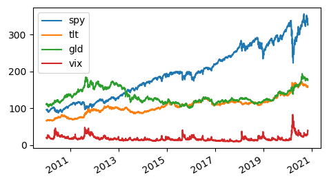
In the previous installments, we presented the concept of Modern Portfolio Theory. We also provided an optimization algorithm, written in Python, for searching for the optimal portfolio.
To continue, we are going to perform some numerical experiments. Specifically, we are going to use the portfolio optimization program developed in the previous post in order to study the effect of diversification.
In finance, diversification is the process of allocating capital in a way that reduces the exposure to any one particular asset or risk. A common path towards diversification is to reduce risk or volatility by investing in a variety of assets. If asset prices do not change in perfect synchrony, a diversified portfolio will have less variance than the weighted average variance of its constituent assets, and often less volatility than the least volatile of its constituents.
... Every equally weighted, uncorrelated asset added to a portfolio can add to that portfolio's measured diversification. When assets are not uniformly uncorrelated, a weighting approach that puts assets in proportion to their relative correlation can maximize the available diversification. Read more
It’s well-known that if we add an asset that is negatively correlated with the existing assets in the portfolio, then it will likely result in a higher risk-adjusted return, i.e. a higher Sharpe ratio. For this reason, in the previous examples, Gold was included as a diversifier.
In this post, we expand our 3-ETF portfolio by adding volatility-related instruments that are known to be negatively correlated with the equity market. We will use our Python program and explore whether the inclusion of a negatively correlated asset would enhance the portfolio’s risk-adjusted return.
Adding VXX ETF
We first add VXX, a volatility Exchange Traded Fund, to the portfolio and run the Python program. The picture below shows the optimal portfolio’s composition and the Sharpe ratio.
![]()
It’s interesting to note that the program determined the weight of VXX to be zero, and consequently, the Sharpe ratio is unchanged. This is probably because the return of VXX is too negative (-66% per annum) so there is no benefit of adding it to the portfolio. Also, the volatility of VXX is high, and adding a volatile asset to a portfolio is not diversification.
Adding spot VIX
We next add spot VIX to the portfolio. Note that spot VIX is not a tradable asset. We do this exercise merely for the sake of numerical experimentation.

The figure below shows the optimal portfolio’s composition and the Sharpe ratio. This time we obtained indeed a higher Sharpe ratio (an increase from 1.17 to 1.45). It’s interesting to note that Gold is now eliminated from the portfolio.
![]()
In summary, this post is an exploration of how to use the optimization algorithm to study the effect of diversification. Readers are encouraged to experiment with other asset classes.
Last and not least, do not forget the assumptions of the Modern Portfolio Theory.
Click on the link below to download the Python program and data files.
Originally Published Here: Modern Portfolio Theory-Effect of Diversification on the Optimal Portfolio-Portfolio Management in Python

No comments:
Post a Comment