Bond Market vs Stock Market

Investors have the option to invest in various assets. Among these, the most well-known are bonds and stocks. The reason behind their popularity is the balance between the risks and rewards they provide to investors. However, both are different from each other in their characteristics and the markets or brokers that contribute to them.

What is a Bond Market?

A bond market is also known as the credit or debt market. It refers to the market in which investors trade debt instruments, most prominently bonds, often issued by companies or governments. When investing in these instruments, investors take the role of a lender. They provide a loan to the issuer of the bond in exchange for subsequent interest and principal payments.

The most prominent advantage of investing in the bond market for investors is that it provides a steady income source. In comparison to stock investments, the income from bonds may be lower. However, it also comes with lower risks for the investor. For government-issued bonds, such as Treasury bonds, the risks may be minimal.

There are various reasons why investors prefer to include bonds in their portfolios. Most prominently, bonds allow them to diversify their portfolio. Similarly, investors prefer bonds in uncertain times, as it provides them with a fixed income with lower risks. Usually, risk-averse investors favour bond investments over other types of investments.

Unlike most stock markets, bond markets don’t have a centralized location. Therefore, investors usually get bonds through a broker-dealer network. Most bond markets don’t have individual investors either. They include larger institutional investors instead. Some of these investors then further trade with individual investors.

What is the Stock Market?

A stock market is a market in which investors trade equity instruments, usually stocks. However, it may also include options and futures. By investing in the stock market, investors can buy shares for the ownership of corporations. As opposed to bond investments, stock investments may provide much higher returns, although they may come with higher risks.

Stock markets are usually centralized locations that bring buyers and sellers together. They provide a regulated and controlled environment where investors can trade with each other or with companies. The transactions involved in the stock market are relatively more transparent and fairer. Therefore, it provides all investors with similar conditions in which they can trade.

The reason why investors prefer to include stocks in their portfolios is that they provide better returns. Investors can not only benefit from steady dividend payments but also take advantage of capital gains. Similarly, stocks have a higher chance of increasing wealth to the holders compared to a bond's fixed-income returns.

What are the differences between a Bond and Stock Market?

As mentioned, the primary difference between the two types of markets is their location. While bond markets are decentralized, stock markets have a centralized location. Similarly, both vary due to the risks involved in investing in their underlying instruments. Likewise, the rewards that investors get from each type of instrument in these markets also differ.

Conclusion

Bond markets are locations where investors can trade debt instruments. On the other hand, stock markets are for equity investments. Investors can use both markets to create a diversified portfolio. However, there are some differences between the markets and their underlying instruments, as discussed above.

Originally Published Here: Bond Market vs Stock Market

What is a Market Index

What is a Market Index?

A market index is a portfolio of securities that represent a segment of the stock market. These securities come with specific characteristics and are a part of a particular stock market index. The value of the index comprises the price of the underlying holdings. However, a market index isn't a real portfolio but rather a hypothetical one.

The most well-known stock indexes in the US market are the S&P 500, Nasdaq Composite, and Down Jones Industrial Average. These represent a collection of stocks from various companies valued based on specific characteristics. Investors can’t directly invest in these indexes, though. However, they can invest in index funds that use these indexes as a benchmark.

How does a Market Index work?

As mentioned, a market index represents a segment of the financial market. Therefore, it measures the value of a portfolio holding that has a specific market characteristic. There are several methodologies used to calculate the value of an index, maintained by the index's provider. Most market indexes use a price or market-cap based methodology.

Investors use market indexes to follow the financial markets and manage their portfolios. Similarly, most funds, such as index funds or exchange-traded funds, use indexes as benchmarks to compare performance. Therefore, market indexes play a critical role in the investment management business.

How is the value of a market index calculated?

There are various market index methodologies used to calculate the value of an index. The value of the index comes from the weighted average calculation of the values of the total portfolio. There are various bases for valuing an index, for example, market-cap weighting, float-weighting, fundamental-weighting, and revenue weighting.

Based on the basis used for valuing an index, an index's value will change with a change in that value for its underlying stock. For instance, the value of a market-cap weighted index will change if the market capitalization of the underlying stocks changes. As the value of an index depends on weighting several stocks, the largest stocks will influence the index's value, more than the smallest ones.

What are the uses for Market Indexes?

Market indexes have several uses or functions. Firstly, investors and portfolio managers can use market indexes as benchmarks.  It is especially true when they perform performance comparisons and making decisions related to investments. Similarly, some funds, such as mutual or index funds, use market indexes as a benchmark.

Market indexes are also commonly used as a method of investing in stocks with similar characteristics. For example, investors usually invest in high-growth potential emerging sectors using market indexes. The use of market indexes also depends on the type of index and its basis.

Lastly, investors can also use market indexes when devising a diversification strategy. Investing in indexes help investors to diversify their portfolio as compared to investing in individual stocks. Similarly, investors can invest in multiple indexes to even further diversify their portfolios. Index investing companies with higher returns but at the same time, lower risks.

Conclusion

A market index represents a hypothetical portfolio of securities that come from a segment of the stock market. The underlying securities within a market index come with specific characteristics. There are multiple methodologies for valuing market indexes.

Post Source Here: What is a Market Index

Asset Allocation and Diversification

When it comes to implementing an investment portfolio, there are two crucial strategies that investors can use. These are asset allocation and diversification. Both of these strategies correlate the risks taken by investors in their portfolio for their given risk tolerance. Similarly, investors can limit their exposure due to risk due to concentrating all their investments in one asset using these strategies. Investors need to differentiate between these strategies to understand them better.

What is Asset Allocation?

Asset allocation helps investors balance their risks and reward by apportioning a portfolio's assets according to various factors. In other words, asset allocation refers to the strategy in which investors divide their investment portfolio between several diverse asset classes to minimize the risks associated with their investment. There are three primary asset classes from which investors can choose, equities, fixed-income, and cash and equivalents.

When considering an asset allocation strategy, investors must consider various factors, as stated. Firstly, investors must consider their goals, which will dictate the risks and rewards they expect. Similarly, they must also regard their risk tolerance level. Lastly, investors also need to consider the time horizon of their investments.

Most experts suggest that investors must reduce their level of volatility of portfolios. Therefore, investors need to diversify their investment into various asset classes. Since every asset class has its own associated risks and rewards, the investors will achieve a diversified portfolio. Similarly, by investing in several asset classes, they can guard against any unforeseen circumstances in a better way.

The idea behind asset allocation is that when investors include various asset classes in their portfolio, a downturn in one asset class will not affect them in the same manner as if they had invested in a single class. By using asset allocation, investors can get compensated for the downfall of one asset class with an upturn in another one.

What is Diversification?

Portfolio diversification isn’t a new topic in the world of investing. It refers to the process in which investors include a wide variety of investments within their portfolio. The goal of diversification is to minimize the unsystematic risk of an investment. Therefore, the negative performance of one investment cannot affect the investors' whole portfolio.

Diversification is different from asset allocation. With asset allocation, investors include investments from different asset classes in their portfolio. On the other hand, diversification applies to a single asset class. Therefore, if an investor buys only stocks of various companies or industries, they employ the diversification strategy, not asset allocation.

However, by diversification, investors cannot guarantee against a loss. Diversification helps in reaching a long-term financial goal while also minimizing risks. The idea behind diversification is that by having various stocks from several sources, investors don't have to suffer due to an unforeseen event that can affect a specific investment or industry. However, that doesn't mean they can protect their portfolio against events that affect the market as a whole. For that, they must use asset allocation.

Conclusion

Asset allocation and diversification are two strategies that investors use to manage their portfolios. While both are a crucial part of investing, there are some differences between both. Given above is a detailed analysis of what they are and how investors can use them in their portfolio management.

Article Source Here: Asset Allocation and Diversification

Monte Carlo Simulation in Excel

What is a Monte Carlo Simulation?

A Monte Carlo simulation refers to a technique used in financial modeling to determine the probability of various outcomes in a process or problem that is not easily predictable or solvable. The reason behind the difficulty of the process or problem is the existence of random variables. A Monte Carlo Simulation produces a simulation based on random samples to achieve numerical results.

While there are various ways to perform Monte Carlo simulations, the easiest way is through Excel. There are various built-in tools in Excel that help with the simulation. The most common tool used in this regard is the "What-If Analysis" tool.

Monte Carlo Simulation in Excel

A company wants to calculate its profits for a project based on estimations. However, there is some uncertainty around the estimates. Therefore, the company performs Monte Carlo simulations. It has the following information available.

	Sales	Cost of Sales	Fixed costs
Expected	1,000,000	350,000	500,000
Standard Deviation	80,000	25,000	120,000

The company assumes there is a normal distribution around these inputs. Therefore, it can perform the simulation using Excel. The first step to perform Monte Carlo simulations is to calculate the normal distribution for the figures above. The company may use the following formula to calculate a normal distribution for all these.

NORM.INV(probability, mean, standard deviation)

For the first parameter, the company uses a random probability using the ‘rand()' function. For the mean parameter, the company uses the expected results. Based on these, the company gets the following outputs.

	Sales	Cost of Sales	Fixed costs
Expected	1,000,000	350,000	500,000
Standard Deviation	80,000	25,000	120,000
First simulation	978,986	385,896	251,134

The company's expected profits, based on the first simulation, will be $341,956.

The next step the company takes is to make a table for the number of simulations it wants to make. For this purpose, the company wants to generate 30 simulations.

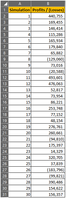
Once it creates a table for the 30 simulations, the company links the profits to the table, from the first simulation. For the other 29 simulations, it uses the What-if Analysis Data Table feature. The tool needs at least one input cell for random calculations. However, the cell should be a cell outside the table. Here's how it looks.

Based on the calculation, it produces the following table.

Based on these simulations, the company performs several other calculations, such as calculating the mean value, which comes to $139,246. The formula it uses is “=AVERAGE(B2:B31)". Similarly, the company measures the standard deviation for the simulations using the formula "=STDEV(B2:B31)”, which comes to $171,670.

Therefore, using excel can help in performing Monte Carlo simulations when there is uncertainty involved in variables. While the above example considers only 30 simulations, users can choose to generate even more simulations based on their needs.

Similarly, the company used the simulation to calculate the average and standard deviation of the outcomes. However, users may use the simulation in more complex ways than that above.

Conclusion

Monte Carlo simulation is a technique used to determine the probability of various outcomes for complex processes in the presence of random variables. While several tools can perform simulations, the most commonly used one is Excel. The Excel feature that helps with Monte Carlo simulations is the What-if Analysis Data Table tool combined with the “NORM.INV” formula.

Article Source Here: Monte Carlo Simulation in Excel

Passive Management vs Active Management

When it comes to investing strategies and managing their portfolios, investors have two main options. They can either use an active or passive management strategy. Both of these strategies have their advantages and disadvantages. However, investors must choose their own tactics that suit them.

To know which option is the best for them, investors need to understand what they are and how they can use it to their benefit.

What is Active Management?

Active management refers to the trading strategy in which investors actively manage their portfolios. Investors using this management strategy buy and sell stocks in order to outperform a specific index, such as the S&P 500 or the market as a whole. Usually, a portfolio manager takes care of the actively managed stocks under this strategy.

Whether investors succeed or fail in this strategy depends on how much research they have performed and the techniques they use. Investors can combine various models and methods to identify stocks that they believe will help them outperform the market. With this management strategy, investors need to identify any opportunities and exploit them readily.

Usually, investors using this investing strategy follow market trends, changes in the political landscape, shifts in economics, legal factors, one-off events, etc. These are the factors that can affect the performance of a specific stock in the market. Based on this research and the data collected in this step, investors can select stocks that they believe are undervalued and may result in profits.

As mentioned, the goal of this strategy is to identify investments that can outperform the market. Therefore, investors will look for the highest possible returns. However, that also means that they will have to bear higher risks compared to other strategies.

What is Passive Management?

Passive management is the opposite strategy for active management, sometimes also referred to as index fund management. In this strategy, investors don't actively manage their portfolio but rather take a passive approach. The goal of this strategy isn't to beat the market but to imitate a particular market index's returns.

Therefore, the purpose of stocks included in a passive portfolio is to generate returns similar to a chosen index. Usually, passive management doesn't require active portfolio managers. Investors using the passive management strategy often prefer investing in mutual funds, index funds, or exchange-traded funds, all of which achieve the goal.

A passive mode of investment is much more inexpensive in comparison, as it does not require proactive management of portfolios. Therefore, the management fees associated with this strategy are minimal. In comparison, active management costs more. However, passive management comes with a downside of lower returns, although it also comes with lower risks.

Which is better, Active Management or Passive Management?

Both types of portfolio management strategies have their advantages and disadvantages. However, it is for investors to decide which one they want to use. Usually, investors consider various factors before choosing a strategy, among which the most critical are time and costs. However, that does not mean investors can't use a combination of both for the best results if they want.

Conclusion

There are two portfolio management strategies that investors can use, active or passive. Active management, as the name suggests, requires proactive portfolio management. On the other hand, the passive mode approach is the opposite.

Post Source Here: Passive Management vs Active Management

Hypothesis Testing in Statistics

What is Hypothesis Testing?

Hypothesis testing is a concept in statistics in which analysts test an assumption regarding a population parameter. It is a method used in statistical inference. The use of hypothesis testing is useful when determining if a statement regarding a population parameter is statistically significant. Overall, it is a critical part of the scientific method, which represents a systematic approach to assessing theories through observation.

Through hypothesis testing, one can assess the plausibility of a hypothesis by using sample data. This data can come from various sources, such as a large population or a process that generates data. Similarly, the hypothesis can come from any judgment used by the user that is achievable. Hypothesis testing is also a great tool for evaluating various scenarios.

How does Hypothesis Testing work?

In hypothesis testing, analysts test a statistical sample to provide evidence on the plausibility of the null hypothesis. To perform hypothesis testing, analysts test a hypothesis by measuring and examining a random sample of the population. They use a random population sample to evaluate two different hypotheses, the null hypothesis, and the alternative hypothesis. The formula for the null hypothesis is as follows.

H₀: µ₀ = 0

Similarly, the formula for the alternative hypothesis is as follows.

H_a = µ₀ ≠ 0

The null hypothesis represents a hypothesis of equality between population parameters. For example, a null hypothesis may state that the population mean return is equal to zero. On the other hand, the alternative hypothesis is the opposite of the null hypothesis, which tests whether the population mean return is not equal to zero.

How to perform Hypothesis Testing?

Hypothesis testing is a several step process. The process starts with analysts stating the null (H₀) and the alternative hypothesis (H_a). After that, they consider the statistical assumptions and whether these assumptions are in line with the underlying population in evaluation. After that, analysts determine the appropriate probability distribution and select the appropriate test statistic.

Then, analysts can select the significance level, which is the probability threshold for which they will reject the null hypothesis. Based on the significance level they use and the appropriate test, they must also state the decision rule. From the testing, they can collect the data observed and use it to calculate the test statistic.

After that, analysts should either reject the null hypothesis or fail to reject it based on the results obtained. The process is called a statistical decision. They must also consider any other economic issues that may apply to the problem. These are non-statistical considerations that they must consider for a decision in addition to the statistical decision for a final decision.

As mentioned, hypothesis testing has two parts, the null hypothesis, and the alternative hypothesis. Analysts try to reject the null hypothesis. That is because the alternative hypothesis is often difficult to prove. So, if the null hypothesis is false, then the remaining alternative theory gets accepted.

Conclusion

Hypothesis testing is a method in which analysts test an assumption about a population parameter. There are two parts to hypothesis testing, testing the null and alternative hypotheses. Performing hypothesis is crucial and consists of several steps, as stated above.

Article Source Here: Hypothesis Testing in Statistics

Confidence Interval in Statistics

What is Confidence Interval?

The confidence interval, in statistics, represents an estimate of an interval that may consist of a population parameter. In other words, it refers to the probability of a population parameter falling between a set of values for a particular proportion of times. A confidence level is a term often associated with sampling because it helps calculate the degree of uncertainty or certainty in a specific sampling method.

There are two limits to the interval which define it. The confidence interval comes in the form of a percentage, which has an upper and lower bound. These percentages reflect the confidence level.

What is Confidence Level?

Confidence level refers to the percentage of probability or certainty that the confidence interval consists of the true population parameter when a random sample gets drawn many times. A confidence level of 0% shows that there is no certainty that the sample includes a true population parameter and, therefore, will draw a different sample each time. A confidence level of 100%, on the other hand, shows that no matter how many times the simple get drawn again, it will result in the same selection.

How to calculate the Confidence Interval?

It is necessary to determine the criteria for testing first to calculate the confidence interval. The confidence interval varies based on the chosen criteria. Next, it is crucial to select a sample from a given population. The sample helps in testing or performing the hypothesis. Next, it is necessary to determine the mean and standard deviation for the sample chosen.

From the given data, it is straightforward to calculate a confidence level. It may range from 90% up to 99%. After calculating the confidence interval, it is also possible to calculate the confidence coefficient for the confidence interval chosen. The calculation of the confidence coefficient is straightforward using z-tables. Finally, it is also possible to determine the margin of error for the estimation.

By using the above information, the confidence interval for the chosen sample with the confidence level becomes determinable. The formula to calculate the confidence interval is as below.

Confidence level = Mean of sample ± Critical Factor x Standard deviation of the sample

How to interpret the Confidence Interval?

Most users of the confidence interval often misinterpret or misuse it. Even most professionals or scientists don't interpret it correctly. For example, a 99% confidence level does not imply that for a given realized interval, the probability that the population parameter lies within the interval is 99%. In fact, for any confidence level, users tend to misinterpret it as the probability of population parameter lying within the interval.

It is one of the most common misconceptions involving confidence level. After calculating the confidence interval, there is no longer a probability of covering the confidence level. It either includes the parameter value, or it doesn't. That is why the confidence interval varies for various samples while the true population parameter doesn't, regardless of the selected sample.

Conclusion

Confidence interval is a term used to represent the estimate of an interval that consists of a population parameter. It is a term closely related to the confidence level, which refers to the percentage of probability or certainty that the confidence interval consists of the true population parameter.

Post Source Here: Confidence Interval in Statistics

Hedging Market Risks Using Volatility Estimators-Are Sophisticated Methods Better?

Previously, we elaborated on why hedging is an important tool for risk management. We illustrated the importance of hedging with examples from the commodity, mortgage back securities, and foreign exchange markets.

A recent paper [1] evaluated the hedging effectiveness of various range-based volatility estimators. Among them, we can find the commonly used GARCH model.

Generalized AutoRegressive Conditional Heteroskedasticity (GARCH) is a statistical model used in analyzing time-series data where the variance error is believed to be serially autocorrelated. GARCH models assume that the variance of the error term follows an autoregressive moving average process.

Although Generalized AutoRegressive Conditional Heteroskedasticity (GARCH) models can be used in the analysis of a number of different types of financial data, such as macroeconomic data, financial institutions typically use them to estimate the volatility of returns for stocks, bonds, and market indices. They use the resulting information to help determine pricing and judge which assets will potentially provide higher returns, as well as to forecast the returns of current investments to help in their asset allocation, hedging, risk management, and portfolio optimization decisions. Read more

The article concluded,

The study is based on weekly data from January 2000 to December 2016 for six markets, including crude oil, gold, silver, natural gas, S&P 500, and NIFTY 50. The performance of hedge ratios estimated with various methods is evaluated with variance and semi-variance as the measures. The empirical results indicate that there is no specific econometric method, which outperforms the others consistently and significantly. The rolling OLS and BEKK GARCH methods are more efficient for estimating the optimal hedge ratio as compared to the other methods. The hedge ratios estimated with range-based models are not as efficient as those estimated with returns-based models are. More importantly, there is no significant difference in the variance/semi-variance of the naïve or rolling OLS based portfolios when compared to the other best-performing portfolios. The results are in line with some previous studies, which suggested that the simple naïve and OLS methods perform as well as the other more complex and sophisticated methods, if not better than them. The range-based methods are no exception to these general findings.

Briefly, simple hedging methods work as well as other more complex and sophisticated ones.

 

References

[1]  V. Pandy, V. Vipul,  Hedging performance of range-based volatility estimators, Journal of Business and Economic Studies, 2020

Article Source Here: Hedging Market Risks Using Volatility Estimators-Are Sophisticated Methods Better?

What is Monte Carlo Simulation

What is Monte Carlo Simulation?

Monte Carlo Simulation is a method from statistics used in financial modeling used to determine the probability of various outcomes in a process or problem that is not easily predictable or solvable because of the existence of random variables. The simulation produced by this model depends on random samples to achieve numerical results.

Monte Carlo simulation can help investors understand the effect of uncertainty and randomness in forecasting models. Similarly, it helps them determine the impact of risk and uncertainty in their modeling or forecasting. The model works by assigning multiple values to random or uncertain variables in order to achieve various results. From these results, investors can calculate an average to obtain an estimate.

The model also has application in various other fields of life, including finance, investing, engineering, science, etc. Another name used to describe it is multiple probability simulation. In finance and other fields related to it, the Monte Carlo simulation assumes a perfectly efficient market.

How does Monte Carlo Simulation work?

Monte Carlo simulation suggests that one cannot calculate or determine the probability of varying outcomes due to the interference of random variables. Therefore, the simulation focuses on constantly repeating random samples to achieve specific results. The basis for it is that it takes variables with uncertainty and assigns a random value to them.

Using that as a basis, the model runs and provides results. The model then repeats calculating and providing outcomes several times while assigning the variable with multiple values. At the end of the simulation, all the results will have different values. To obtain an estimate from those results, users must average them.

How does Monte Carlo Simulation help in finance and investing?

The Monte Carlo simulation has various applications in the finance sector and for investors. Firstly, investors can use it to evaluate or weigh different investments. Most commonly, they use it in equity options pricing. It can help investors estimate the current value of an option by simulating different paths for the price.

Monte Carlo Simulation can also help investors in portfolio valuation. Any factors that can play a role in the valuation of a portfolio get simulated, which helps in the calculation of portfolio value. After that, investors can find the average value of all the simulated portfolios to get a final portfolio value. It can also help in financial modeling, as stated above.

Lastly, the Monte Carlo simulation helps in the valuation of fixed income instruments and interest rate derivatives. The primary source of uncertainty for those instruments or derivatives is the short rate. The simulation helps assign a number to the short rate and simulate results to obtain the price of a bond or derivative for each rate. In the end, it helps in evaluating them by calculating an average of the obtained results.

What are the limitations of Monte Carlo Simulation?

Monte Carlo simulation has various limitations. Firstly, it does not provide exact results but rather statistical estimates of results. Similarly, the simulation is complex and may require costly software specially designed to carry out the complex simulations. Lastly, due to its complexity, the process of simulation may cause various errors which can produce inaccurate results.

Conclusion

Monte Carlo Simulation is a method used to determine the probability of various outcomes in an unpredictable or unsolvable problem because of uncertain variables. The model is complex but can help in finance and investing, such as financial modeling, evaluating investments, portfolio valuation, etc.

Post Source Here: What is Monte Carlo Simulation

Variance and Standard Deviation

Variance and standard deviation are two fundamental concepts in mathematics that have a vital application in the worlds of finance, economics, investing, and accounting. In investing, investors use these to devise a plan for their investments. It can help them build an attractive portfolio by developing an effective trading strategy.

What is Variance?

The variance relates to the mean, which is the average of a group of numbers. The term variance gives a measure of the average degree to which numbers within a set differ from the mean. Furthermore, the extent of the variance correlates to the size of the overall range of numbers. It means the more spread the range of numbers in a set are, the greater the variance is as well. On the other hand, the variance for a narrower range of numbers will be less.

Mathematically, the variance refers to the average of the squared differences from the mean. When users want to calculate it, they must calculate the mean of a set of numbers. After establishing the mean, they must calculate the difference between each element in the set and the calculated mean. Lastly, they need to square and average the results.

What is Standard Deviation?

Standard deviation is a statistic that gives a measure of how far a group of numbers is from the mean. The standard deviation, mathematically, is the square root of the variance. To calculate variance, users need to use squares because it gives more importance to outliers than any data that is closer to the mean. The calculation allows for the difference about the mean from canceling out those below, which may result in zero variance.

The calculation of standard deviation requires calculating the variation between each value in a set relative to the mean. If the difference between a number and the mean is high, there is a higher deviation. Similarly, if the difference is low, there is a lower deviation. Therefore, for a set that has a spread group of numbers, the standard deviation will be higher.

Therefore, to calculate standard deviation, users need to add up all the data points first and divide them by the number of data points. In other words, they need to calculate the average for the set of data points. Then, they need to calculate the variance for each data point. Lastly, they can square root the variance to get the standard deviation.

How do Variance and Standard Deviation help in investing?

Both variance and standard deviation have significant importance for investors. They are crucial when investors want to calculate the security and market volatility of a stock. By identifying or calculating these, investors can develop an effective and profitable trading strategy and diversify their portfolios.

Standard deviation also helps investors measure the risk associated with an investment. When the group of numbers in the considered set are close to the mean, it represents a less risky investment. In other words, a low standard deviation represents a lower risk investment as compared to a high standard deviation. However, high-risk investments may indicate better returns.

Conclusion

Variance and standard deviation are concepts used in mathematics that have a paramount significance in the world of finance and investing, among others. The term variance represents the measure of the average degree to which numbers within a set vary from the mean. On the other hand, the standard deviation shows how far a group of numbers with a set are from its mean.

Post Source Here: Variance and Standard Deviation

Formula for Expected Value

What is Expected Value?

Expected value refers to the anticipated value of a variable. It represents a generalization of the weighted average of a variable. Other names used for the expected value of a variable are expectation, mean, average, first moment, or mathematical expectation. While mostly associated with economics and statistics, the expected value is also crucial in finance and investing.

The calculation of expected value involves aggregating the product of the likelihood of an outcome occurring with each of the possible outcomes. For example, for four different outcomes, it is necessary to calculate what the probability of each outcome occurring is and then to multiply the product of those likelihoods with the outcomes. Then it is critical to sum all the results to get an expected value.

How does Expected Value apply in finance and investing?

In investing, investors usually use expected values to estimate a value for an investment in the future. For a random variable, its EV gives a measure of its center of the distribution. Similarly, calculating an expected value allows investors to evaluate various scenarios and choose the one most likely to achieve their desired output.

Therefore, it is a crucial concept used in scenario analysis, which is a technique for determining the expected value of an investment opportunity. Investors can not only calculate the expected value of single discrete variables but also for single continuous, multiple discrete, and multiple continuous variables. Therefore, it is also common to use expected values with multivariate models.

What is the formula for Expected Value?

The formula to calculate the expected value for a single event that repeats multiple times is straightforward, which is as below.

EV = P(X) x n

In the above formula, 'P(X)' represents the likelihood or probability of the event occurring, while 'n' shows the number of times the event will repeat. It is the simplest form of expected value. However, in investing, the calculations are more complicated and often involve multiple events. In these cases, the formula for expected value changes to compensate for multiple events, as below.

EV = ∑P(Xi) x Xi

In the above equation, ‘P(Xi)’ represents the probability of the event and ‘Xi’ denotes the event. However, the difference between the two formulas is that of the summation of expected values. In this case, investors must calculate various expected values for multiple events and aggregate them to get a probability-weighted average.

Example

An investor wants to decide between investing in two stocks. The first stock has a 60% chance of achieving a $1,000 return, while a 40% chance of getting a $500 return. On the other hand, the other stock has a 20% chance of a $2,000 return while an 80% chance of $400. To select the best option, the investor can calculate the expected value of both stocks and compare them with each other.

For the first stock, the expected value would be as follows.

EV = [60% x $1,000] + [40% x $500]

EV = $800

For the second stock, the expected value is as follows.

EV = [20% x $2,000] + [80% x $400]

EV = $640

According to the expected values of both stocks, the best option for the investor is to go with the first option.

Conclusion

Expected value is a concept used in statistics to represent the anticipated value of a variable. In finance and investing, it can help investors in estimating the value of an investment in the future. It is a concept that is the core of scenario analysis and multivariate models.

Originally Published Here: Formula for Expected Value

Median Meaning in Math

What is Median?

In mathematics, the median represents the middle point of a sorted list of numbers. In a way, it shows the average of a given set of numbers. For example, for a random set {12, 13, 18, 10, 5, 2, 9, 6, 15, 14, 3}, the median will be the number '10'. In order to find the median in the above set, it is necessary to sort the list first. The sorted list, in this case would be {2, 3, 5, 6, 9, 10, 12, 13, 14, 15, 18}.

From the sorted list given above, the median would represent its middle point. Since there are a total of 11 numbers in the list, the median would be the 6^th element of the list. In the sorted list, the 6^th element is the number '10'. Therefore, it is the median of that particular given set of numbers. As mentioned, however, the list must be sorted first.

The above set of numbers contains an odd number of elements. Therefore, the median for the list is only a single number. The number, in that case, '10', represents the central point of the sorted listed that has an equal number of elements above and below it. However, when a list contains an even number of elements, the median will be the average of the pair of numbers that fall in the middle.

Along with mean and mode, the median is a critical concept used to derive the average of a given set of data points. While the median represents the midpoint of the set, the mean and mode calculate the average differently. Another name used for the median is positional average, which gives an accurate description of what it is.

What are the uses of Median?

There are several uses of the median. Most commonly it can be used as a measure of location in cases where the extreme values of a given set of elements have low importance, usually due to a skewed distribution. Similarly, it helps when the extreme values of a set are unknown or when the anomalies or outliers are untrustworthy.

For example, in the set {5, 20, 22, 22, 23, 23, 43}, the mode is 22, which is a better representative of the positional average of the set. In the case of the given set, both the extreme ends (5 and 43) may represent extreme values that are untrustworthy due to how different they are from the average.

Similarly, the median is simple to understand and easy to calculate. However, that does not take away from its usefulness and application in mathematics and other fields. It is one of the most well-known summary statistics in descriptive statistics while also being a robust approximation to the mean.

Can Median help in finance and investing?

In finance and investing, the median can also have an application, especially during comparable analysis. When comparing between stocks of different nature, investors may want to neglect the extreme values that they consider untrustworthy or are significantly different from the average of the given data. In that case, using other ways to calculate the average may not produce a representative result.

However, by using the median, investors can easily avoid the problem and get a representative element that is will give them an idea of the positional average of the given set of data. While the process of determining a median for a large amount of data may be a tedious task, with the use of tools such as Excel, the process becomes simpler. Therefore, any investor can calculate a median for their data if they understand what it represents.

Conclusion

Median, in mathematics, shows a positional average or middle point for a set of sorted numbers. For oddly numbered elements in a sorted set, the median is the number above and below which there are a similar number of items. For evenly numbered elements in a sorted set, the median is the average of the pair of numbers that fall in the middle.

Originally Published Here: Median Meaning in Math

Formula for Arithmetic Mean

What is Arithmetic Mean?

The arithmetic mean is a term used in mathematics and statistics to describe the sum of a collection of numbers divided by the count of numbers. Simply put, the arithmetic mean is the average of a set of numbers. The arithmetic mean is a crucial concept in all fields of life, such as science, finance, statistics, economics, etc.

While the arithmetic mean of a set of numbers represents its central tendency, it can be influenced by anomalies or outliers in the given set. Therefore, for a skewed distribution, the arithmetic mean may not be truly representative of the midpoint. On the other hand, other statistics, such as the median, provides a much better representative midpoint because it ignores the extremes in a set.

What is the formula for Arithmetic Mean?

The formula to calculate the arithmetic mean of a set of numbers is straightforward, which is as below.

Arithmetic Mean = (a₁ + a₂ + a₃ + … + a_n) / n

In the above formula, 'a_n' represents the value of the nth number in a given set. On the other hand, 'n' denotes the count of numbers in the set. In order to calculate the arithmetic mean of numbers in observation, it is necessary to calculate the sum of those numbers first. By putting the sum in the above formula and dividing it by the count of the elements in the observation, one can get its arithmetic mean.

How does Arithmetic Mean help in finance and investing?

The arithmetic mean is a crucial concept in the world of finance and investing. For instance, investors can estimate their mean earnings using the arithmetic mean formula. Similarly, they can calculate the average returns on several stocks. Furthermore, investors can use it to calculate a stock’s average closing price during a particular period.

The most important advantage of using the arithmetic mean in the world of finance and investing is that it is straightforward to calculate and comprehend. Any investor with even basic knowledge of mathematics can calculate the arithmetic mean for different aspects of a given stock or investment. It is useful in calculating or estimating the central tendency providing more valuable results even if there are a large number of elements.

What are the limitations of Arithmetic Mean?

The arithmetic mean does not always produce the best results, especially in cases when anomalies or outliers exist in a given set. These outliers can skew the average or mean substantially. As mentioned, in these cases, there might be better measures or formulas to calculate a closer central tendency instead of using the arithmetic mean.

In other cases, such as when investors need to calculate the performance of their investment portfolios, especially when it consists of compounding or reinvestments, arithmetic mean can be futile. Similarly, it may not produce the best results when calculating present and future cash flows used by analysts in making estimates. Using arithmetic mean in these circumstances can produce inconsistent results.

Conclusion

Arithmetic is a concept in mathematics that describes the sum of a collection of numbers divided by the count of numbers in a set. It is useful in finance and investing and is used to calculate various averages. However, it may have some limitations as well.

Post Source Here: Formula for Arithmetic Mean

What is Survivorship Bias

For processes that involve analyzing a high amount of data, sampling is a critical process. However, for it to be effective, the user must select the sample properly. Nonetheless, it might not be possible to do so because some bias may exist when users choose a sample from a given population. There are various types of biases that cause users to select the wrong sample.

What is Survivorship Bias?

Survivorship bias is a type of bias caused during sampling selection. It occurs when investors only consider the surviving or existing observations but fail to take into account data that no longer exists. Practically, survivorship bias happens when investors examine the performance of only existing stocks in the market and regard them as a representative sample while disregarding stocks that have gone bust.

When the process of sample selection gets affected by survivorship bias, it can result in wrong decisions made by investors. For example, by not considering stocks that no longer exist, investors miss out on vital information on what caused those companies to cease. There are multiple factors that investors miss through survivorship bias in their decision-making.

How does Survivorship Bias affect investors?

Survivorship bias makes investors select samples that show a positive view of the market while avoiding its negative aspects. This bias exists because it only considers optimistic samples that have survived due to their steadfastness in strenuous conditions but do not consider those that failed in similar conditions. By not considering the failures, investors make decisions only based on successful histories.

A sample selection based on survivorship bias does not show the whole picture. While the existing data is what investors need to make decisions about, they also need to consider the other failed items in the population to get a representative sample. Furthermore, survivorship bias also causes the results of the analysis performed by investors to skew higher.

How to prevent Survivorship Bias?

Preventing survivorship bias is straightforward. When making a selection of samples, investors need to be aware of its existence. Therefore, they need to not only consider the successful stocks or samples but also look for items that they would not examine. Similarly, investors need to review their data sources to ensure they present both surviving and non-surviving data about their analysis.

Another way to prevent survivorship bias is for investors to not rely too heavily on past returns when making their decisions regarding investments. When investors have a limited view while performing analysis, they are bound to miss vital information during the process. Similarly, they need to ensure they select a representative sample in the selection process.

Example

An investor considering investing in mutual funds comes across the following data.

Mutual Fund no.	Historical return	Active/inactive
1	5%	Active
2	-3%	Inactive
3	7%	Active
4	-4%	Inactive

If the investor considers the active mutual funds only, their average return will be 6%. However, if they vet the inactive mutual funds in the equation as well, the average return would be 1.25%. Therefore, their decision-making can substantially change by considering those non-existent mutual funds along with active ones. If they don't evaluate the inactive mutual funds, it results in a sample selection based on survivorship bias.

Conclusion

In investing, survivorship bias occurs when investors fail to consider the data that is no longer active. For example, when investors fail to take into account the stocks that no longer exist when selecting a sample of stocks. Survivorship bias can have negative impacts on the decision-making of investors. However, it is still preventable.

Article Source Here: What is Survivorship Bias

Data Mining Bias

The selection of an appropriate sample size is often a debatable topic. When selecting samples, it is crucial to choose correctly, so that the results obtained are not biased. However, many issues can result in a biased selection of samples and, therefore, result in a lower quality of parameter estimates.

Usually, when the sample size is large enough, then the chances of bias in sample selection resulting in inaccurate results minimize. With a large enough sample size, one can assume all the distributions will be normal. However, the main challenge is when the size of the sample is small and has a non-normal population.

What is Data Mining Bias?

Data mining bias occurs when investors go through a dataset in order to identify statistically significant patterns, which may come as a result of a random or unforeseen event. Therefore, data mining bias results in investment strategies that are unsuccessful in the long run. This type of bias usually occurs during the research process when investors try to put weight on identifying patterns.

The more investors are biased while mining data, the more inaccurate results they will get in the long run. Similarly, any decisions based on the data affected by this type of bias can also produce negative outcomes. The basis for most inaccurate investing decisions made by investors comes from data affected by data-mining bias.

What is Data Mining?

Data mining is a process of research and analysis used to process a significant amount of data or information. In investing, data mining refers to the process that investors use to track movements in the market, identify patterns, and any turns or changes in the market direction. Based on this analysis, investors can shape their decisions and make investments.

Almost all investors around the world use data mining to some extent when making decisions. However, when they start putting weight or importance on any anomalies that may represent one-off events or changes. The problem then arises when the investors act on the data and get a negative or unexpected result.

What causes Data Mining Bias?

There are various reasons why data mining bias may exist. Firstly, data mining bias can come as a result of the favorability of anomalies. When investors look at market data, it will consist of random patterns. However, when investors start examining those events, considering them to be anomalies and placing more weight on them than they deserve, the resultant data will include data mining bias.

Similarly, data mining bias can come as a result of past experiences. When investors exploit a random event to make profits, they will start looking for these types of irregularities. Based on that experience, when investors single out similar events in the hope of achieving the same results, it can result in a data-mining bias.

Therefore, data mining bias can come as a result of too much digging performed by investors when evaluating stock with the hopes of identifying patterns that can generate income for them.

Conclusion

When selecting an appropriate sample size for decision-making, investors can perform a biased selection, which can cause negative results. One such problem comes in the form of data-mining bias, which occurs when investors examine a dataset in order to identify statistically significant patterns, which may come as a result of random events.

Post Source Here: Data Mining Bias

What is Central Limit Theorem

The Central Limit Theorem (CLT) is a concept from statistics, which states that the sample mean distribution of a random variable approaches a normal distribution as the sample size increases. Briefly, it suggests that the sampling distribution of the mean resembles normal distribution with an increase in the size of the sample, regardless of the shape of the original distribution.

For example, a user has a distribution that considers 20 samples. As they increase their size from 20 to 30 or 40, the distribution will approach a normal distribution. The theorem also suggests that a user must consider at least 30 samples for it to be true.

How does the Central Limit Theorem work?

The central limit theorem suggests that the random samples of a random population variable, regardless of its distribution, will approach a normal probability distribution when the sample population exceeds 30. However, as the user increases the number of samples considered, the graph will start resembling a normal distribution more and more.

With the central limit theorem, the average of the sample means and standard deviation will equal the population mean and standard deviation. Therefore, users can utilize it to predict the characteristics of the population.

How can Central Limit Theorem help in finance?

The central limit theorem helps researchers or analysts in predicting the mean and the standard deviation of a population with the help of a sample selected from it. Since it requires a randomly selected sample size of larger than 30, any sample size selected will approach a normal distribution, which further helps in hypothesis testing and constructing a confidence interval for it.

In finance, investors use the central limit theorem when examining the returns of a stock or indices because it helps with easier analysis. Similarly, investors use the theorem when creating their portfolio or managing the risk related to it. The central limit theorem is easy to use as the financial data necessary to construct it is straightforward to obtain.

For example, investors can select any 30 random stocks from an index to predict the population with the help of the sample as it will follow a normal distribution. Similarly, the mean and the standard deviation of the selected sample of stocks will be the same as the mean and the standard deviation of the overall index. Therefore, it can help them with decision-making about investing in the index as a whole.

What are the characteristics of the Central Limit Theorem?

The central limit theorem exhibits a few characteristics. Firstly, the mean of the sample means is equal to the mean of the population from which investors select the sample. Similarly, as mentioned above, the sampling distribution to approximate a normal distribution should have a sample size larger than 30. Lastly, the standard deviation of the distribution of sample means will equal the population standard deviation divided by the square root of the sample size (σ/Sqrt(n)).

Conclusion

The central limit theorem is a topic of importance in statistics. It suggests that the sample mean distribution of a random variable will approach a normal distribution with an increase in the sample size. However, the sample size should be equal to or exceed 30 to achieve a normal distribution.

Post Source Here: What is Central Limit Theorem

What is Normal Distribution

Normal distribution is a term commonly used in the field of social sciences. Another name for it is the Gaussian or Gauss distribution. Similarly, it is also a term closely associated with the Central Limit Theorem. The normal distribution represents a probability distribution that symmetric (having positive and negative values) around its mean. It has two ends or tails, known as the right and left tails.

Graphically, it resembles the shape of a bell with an upward curve in the middle. Normal distribution helps describe all possible values that a random variable may take with a given range. It is the most common type of distribution assumed in the technical analysis of the stock market and other statistical analyses.

What are the parameters of Normal Distribution?

There are two main parameters of the normal distribution, namely the mean and standard deviation. These parameters play an important role in shaping the distribution and determining its probabilities. The shape of the distribution depends on the values of these parameters.

Mean

The mean is a measure of the central tendency of the distribution. It helps describe the distribution of variables measured as ratios or intervals. For the normal distribution graph, the mean lies at the location of the peak, and most data points reside near it. Any changes in the value of the mean results in the curve shifting to the left or right along the X-axis.

Standard Deviation

Standard deviation represents a measure of the dispersion of data points with respect to the mean. It shows how far away data points reside from the mean and represents the distance between those points and the mean. The standard deviation is associated with the width of the curve rather than its height, unlike the mean. A small standard deviation can create a steep curve while a large deviation produces a flatter curve in the normal distribution.

What are the characteristics of normal distribution?

The normal distribution has several characteristics. Firstly, it is perfectly symmetric, meaning the distribution curve on both sides is equal. Similarly, the mean, mode, and median of a normal distribution are equal. It is because the point of maximum frequency lies in the middle where all three of these exist. Similarly, in most cases, the distribution exists in the center, while fewer values exist at the tail end.

Furthermore, it represents a family of distribution where the mean and standard deviation dictate the shape of the distribution.

How to calculate or graph Normal Distribution?

The formula to calculate the normal distribution is as follows.

X ~ N (µ, α)

In the above formula, 'N' represents the number of observations. 'µ' is for the mean of those observations. Lastly, 'α' represents the standard deviation.

What are the uses for Normal Distribution?

The normal distribution represents an essential statistical concept that can help in financial analysis as well. It helps investors in constructing their portfolios. For example, it can help them identify overvalued or undervalued stock by tracking the movement of price action from the mean. Overall, investors can use it to devise quantitative and qualitative financial decisions.

Conclusion

The normal distribution is a technique used to show a symmetric probability distribution. It has two parameters, a mean and standard deviation. The normal distribution has several characteristics, some of which are discussed above.

 

Article Source Here: What is Normal Distribution

What is Log-Normal Distribution

The log-normal distribution is a term associated with statistics and probability theory. Similarly, another name for the log-normal distribution is Galton distribution. The log-normal distribution represents a continuous distribution of random variables with normally distributed logarithms. It follows the concept that instead of having normally distributed original data, the logarithms of the data also show normal distribution.

A log-normal distribution is similar to normal distribution. In fact, the data in both of them can be used interchangeably by calculating the logarithms of the data points. However, the log-normal distribution is different from the normal distribution in many ways.

The biggest differentiating factor between the two is their shapes. While normal distribution represents a symmetrical shape, a log-normal distribution does not. The difference in their shapes comes due to their skewness. As log-normal distribution uses logarithmic values, the values are positive, thus, creating a right-skewed curve. Another difference between the two is the values used on deriving both.

What are the parameters of Log-normal Distribution?

The log-normal distribution has three parameters. These are the median, the location, and the standard deviation. Firstly, the median, also known as the scale, parameter, shrinks, or stretches the graph, represented by 'm'. Secondly, the location, represented by 'Θ' or 'μ' represents the x-axis location of the graph.

Lastly, the shape parameter or standard deviation, represented by 'σ', affects the overall shape of the log-normal distribution. It does not impact the location or height of the graph. The parameters are available in historical data. However, it is also possible to estimate using current data.

What are the characteristics of Log-normal distribution?

Log-normal distribution has several characteristics or features. First of all, it shows a positive skew towards the right due to its lower mean values and higher variances in the random variables in consideration. Secondly, for log-normal distribution, the mean is usually higher than its mode because of its skew with a large number of small values and few major values.

Lastly, log-normal distribution does not include negative values. It is a feature that differentiates it from a normal distribution and, therefore, a defining characteristic.

What are the uses of Log-normal distribution?

Log-normal has several use cases in the world of finance. Most importantly, it fixes some problems with normal distribution, which helps increase its usage. For example, a normal distribution may include negative variables, while log-normal distribution consists of positive variables only. Apart from that, log-normal distribution is also commonly used in stock prices analysis.

Log-normal distribution can help investors identify the compound return that they can expect from a stock over a period of time. Usually, they use the normal distribution to analyze the potential returns they get from it. However, for analyzing the prices of stocks, log-normal is a better choice.

In finance, log-normal distribution common for calculating asset price over a period of time. It is because normal distribution may provide inconsistent prices, while log-normal does not have the same problem. It solves the problem with normal distribution taking asset prices below zero or negative. Therefore, the log-normal produces better results.

Conclusion

The log-normal distribution shows the continuous distribution of random variables with normally distributed logarithmic values. It is different from the normal distribution in several ways. There are three parameters in log-normal distribution, the median, the location, and the standard deviation.

Originally Published Here: What is Log-Normal Distribution

What is Random Walk

The random walk is a phenomenon used in statistics, which suggests a variable follows no discernible trend and moves at random. It also has an application in trading and finance. In the case of investing, the theory suggests that the changes in stock prices are independent of each other and have the same distribution.

According to this theory, investors cannot use the movement or trend of a stock price in the past to predict its future movement. In essence, the theory suggests that any prediction or estimation based on historical information of stock does not matter as there is no predictable path that the price of a stock can take. Instead, the movement is random.

How does the Random Walk Theory apply to investments?

The random walk theory believes that historical stock prices depended on the information that was available in the past. Therefore, in the present, stock prices are not dependent on historical information because the information available in the present may differ.

Through its efficient market assumption, the theory also suggests the price of a stock will already incorporate any predictions or forecasts related to it. It is based heavily on the premise that investors cannot use techniques that use historical information to predict future outcomes because of the unpredictability or randomness of stock prices.

What does the Random Walk Theory implicate?

The random walk theory by implying that it is not possible to predict the movement of prices, suggests that investors cannot outperform the market in the long run. It, therefore, infers that to outperform the market, investors must take large amounts of additional risk. Furthermore, it does not consider the use of technical or fundamental analysis tools dependable.

What are the advantages and disadvantages of the Random Walk Theory?

There are various advantages and disadvantages that the theory has. Firstly, it provides investors with a cost-effective way of investing in the form of exchange-traded funds. Similarly, many popular predictions and forecasts related to stocks and markets have failed in the past, which further strengthens the suggestion made by the theory.

What are the limitations of the Random Walk Theory?

There are several limitations of the random walk theory. Firstly, it assumes an efficient market in which the prices of stocks reflect all available information. Secondly, it fails to compensate for the fact that the stock market has a large number of participants or investors. Each participant spends a different amount on the market. Therefore, patterns or trends may emerge in the prices of securities in the market.

Through the use of these trends, investors can outperform the market by following the patterns and strategically buying and selling stocks. Similarly, for some stocks, their prices may follow specific trends, even in the long run. Furthermore, some experts believe that several factors affect the price of a stock. Therefore, it may not always be possible to identify it. However, that does not mean a pattern does not exist at all.

Conclusion

Random walk suggests that a variable does not follow a trend or pattern but moves randomly. In finance and investing, the random walk theory suggests that investors cannot use predictive methods to estimate the future price of a stock. Therefore, it believes the use of technical and fundamental analysis tools is futile.

Originally Published Here: What is Random Walk

Linear Regression in Excel

Regression analysis consists of a set of statistical methods often used to estimate the relationship between two variables, one independent and the other dependent. It is a useful tool in several cases, especially for modeling and forecasting. Mostly used in statistics, regression analysis can also be beneficial in finance and investing.

When it comes to regression analysis, there are several variations that one can use. Among these, one is the linear regression analysis.

What is Linear Regression?

Linear regression consists of analyzing two different variables to find a single, linear relationship. Usually, investors use it to determine the relationship between price and time. In this case, time is the independent variable, while the price is a dependent variable that fluctuates with time. Through regression analysis, investors can identify the highest and lowest price points, entry price, exit prices, and stop-loss price.

What are some assumptions for Linear Regression?

There are a few assumptions that investors need to make in order to determine the relationship between two variables in linear regressions. Firstly, investors must assume there are two variables, one of which is independent and the other dependent. For the independent variable, investors must consider it as truly independent. Similarly, investors must also assume the data does not consist of any different error variances.

Lastly, investors must also assume a correlation between variables, which means the error terms of each variable must be uncorrelated. In case any of these assumptions are not true, the linear regression analysis will fail.

How to perform linear regression in Excel?

Linear regression is complicated for investors, as it is a statistical tool. Without the proper knowledge, they cannot perform it. However, with the help of Excel, the process becomes much straightforward. The best way to perform linear analysis using Excel is through the use of charts.

For example, an investor wants to perform linear regression on the price of a stock. They have prepared the following information based on historical prices from the stock market.

Year	Stock price ($)
2015	89.5
2016	93.6
2017	95.7
2018	96.9
2019	102.7
2020	104.6

 

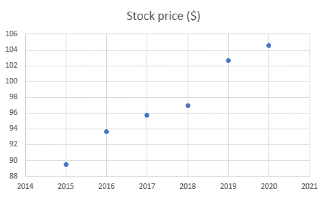
In this case, the independent variable is the year, and the dependent variable is the stock price. Using a chart, the investor can see the changes in the dependent variable in relation to the independent variable. The best chart for this purpose is a scatter chart.

The data must be selected or highlighted to create a scatter chart. From there, the option to create a scatter chart is available under the 'Insert' tab in Excel 2019. It is as below.

It will produce a chart similar to the one below.

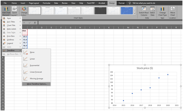
The next step is to generate a trendline. The option to create a trendline is online available if the chart is selected. The trendline option becomes available by selecting the chart and going to the tab and clicking on 'Add chart element'. The easiest way to create a trendline is to use the 'Linear' option from the 'Trendline list'.

However, for Linear Regression, it is critical to click the 'More Trendline Options' option, as shown below.

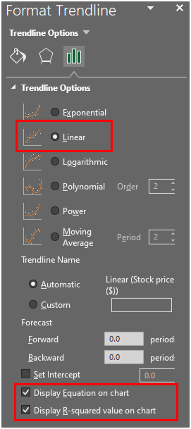
This option will open a new sidebar on the right. By selecting the 'Linear' option from the bar, the chart will display a linear line. From there, the options 'Display Equation on chart' and 'Display R-squared value on chart' will give information related to linear regression, as follows.

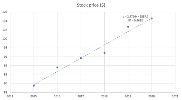
It will give information related to linear regression on the chart. The final chart will look similar to the following.

In the above equation, 'y' signifies the linear regression of the given data. The 'R²' shows the percentage of variance in the dependent variable that the independent variable explains collectively.

Conclusion

Linear regression is a technique used to determine the relationship between two variables. There are some assumptions that investors need to make to use it. The best way to perform linear regression in Excel is through the use of the charts feature, as explained above.

Article Source Here: Linear Regression in Excel

Formula for Moving Average

A tool that investors commonly use to determine the direction of a trend is the moving average. It shows a summary of the data points of financial securities over a specific time. Similarly, it calculates the average for it by dividing the total by the number of data points. The reason it is called moving average is that it continuously changes because the average is recalculated based on the latest price data.

In investing, a moving average is common when it comes to the technical analysis of a stock. Investors use it to help smooth out the price data by calculating an average price continually. It eliminates the impact of any random or short-term fluctuations in the price of a stock over the specified time. Similarly, investors can use the moving average to identify support or resistance by evaluating the movements in a stock's price.

Types of Moving Averages

There are two main types of moving averages that investors can use. These are as follows.

Simple Moving Average

The simple moving average, as the name suggests, is a basic type of moving average. It only considers the recent data points in a given set and divides the total by the number of time periods. Investors use it to determine when to enter or exit a market. Simple moving average only considers historical data. Investors can calculate it for different types of prices, i.e., low, high, open, and close.

The formula to calculate the simple moving average is as follows.

Simple moving average = A₁ + A₂ + … + A_n / n

In the above formula, 'A' represents the average for each period, while 'n' denotes the number of periods.

Exponential Moving Average

The exponential moving average is more complicated compared to the simple method. It gives more preference to the most contemporary price points to make the moving average more responsive to them. Therefore, it is more responsive to the recent price change in the market. However, calculating the exponential moving average requires more work.

To calculate the exponential moving average, investors need to start with the simple moving average for the period. Similarly, they need to calculate the 'multiplier' for weighting the exponential moving average using the formula: [2 / (selected time period + 1)]. Using those, the investor can calculate the current exponential moving average. The formula for the calculation is as below.

Current Exponential Moving Average = [Closing Price - EMA previous time period] x Multiplier + EMA previous time period

Why is Moving Average important?

Moving average is a crucial concept in capital markets for technical analysis of the prices of a stock. Using moving average, investors and analysts can identify any trends in them. They may also use the moving average as lagged indicators as it uses historical information and, therefore, the averages cannot exceed the closing prices. Lastly, moving averages also assist in the calculation of support and resistance level in technical charts.

Conclusion

Moving average is a tool used by investors to define the direction of a trend. There are two types of moving trends that they can use, the Simple Moving Average and the Exponential Moving Average. Both of these produce different results. Overall, moving averages have significant importance, as discussed above.

Article Source Here: Formula for Moving Average

What is Correlation Analysis

Correlation analysis is a tool used to test the relationship between various variables, either quantitative or categorical. It measures how these variables affect each other. Through analyzing the correlation between different variables, making predictions or estimates on future behaviours becomes less complex.

When it comes to investing and finance, correlation analysis is the study of how two securities fluctuate in relation to each other. Correlation is an important concept used in advanced portfolio management. Usually, correlation analysis consists of establishing a 'correlation coefficient' which ranges between -1.0 and +1.0. Investors can also determine a benchmark index and perform correlation analysis with respect to it.

What does Correlation signify?

Correlation signifies how strong the relationship between two quantitative variables through the correlation coefficient. As mentioned above, the correlation coefficient can range from -1.0 to +1.0. A +1.0 coefficient shows a perfect positive correlation. It means that the relationship between the two securities is the strongest. When one security fluctuates, the other security will also follow the exact trend in the same direction.

In contrast, the -1.0 correlation signifies a perfect negative correlation. Here, the correlation is in the opposite direction. Therefore, when one security fluctuates, the other security will also have the same fluctuation but in the opposite direction. For example, if one security goes up, the other will go down. Lastly, a zero correlation shows no correlation at all.

How to calculate the Correlation Coefficient?

Investors can use the formula below to calculate the correlation between two variables.

In the above formula, 'r' represents the correlation coefficient. 'x' denotes the value of the first variable in consideration. 'x̅' indicates the average observations of the first variable. Similarly, 'y' and 'ȳ' show the value of the second variable and its average observations, respectively.

Investors need to follow a few steps when calculating the correlation coefficient. Firstly, they need to obtain a data sample with two variables, which will represent 'x' and 'y'. Similarly, they need to calculate the average or mean for both variables. These will constitute 'x̅' and 'ȳ'. Then they can subtract the mean values from both variables for the formula.

After subtracting both means from their respective variables, investors will need to multiply the residual amounts with each other and find the sum of these multiplications. For the denominator, they will also need to square both of them before calculating the sum. After calculating it, they can square root it and obtain the value of the denominator. Finally, they can divide the nominator by the denominator to calculate the correlation coefficient.

Example

An investor wanting to track the performance of a specific index, for example, Nasdaq Composite, wants to calculate if investing in a company will increase their systematic risk. The investor calculates the correlation coefficient between the stock and the index to be +0.90. It means that the stock has a high positive correlation with the index.

Based on this, the investor understands that the high positive correlation will result in an increase in the systematic risk of their portfolio.

Conclusion

Correlation analysis is the method of testing the relationship between various variables. In investing, investors use it to calculate the correlation of various securities or stocks. Usually, they may calculate the correlation coefficient between a stock and a specific index.

Originally Published Here: What is Correlation Analysis

Is Quant’s Life Hard or Easy?

Last month, efinancialcarreeers published a post, stating that quant’s life is getting harder these days.

Back in the day, a quant in finance could devise a strategy, sit back and let the money roll in while lounging about in a silk robe with a fat cigar. Such are the halcyon dreams of the contemporary quantitative finance type who finds him/herself forced to grind continuously in front of a screen in search of illusory alpha while every man/woman with a piece of Python code does the same.

This wasn't the exact complaint at today's Quant Conference (held digitally this year), but it came close. Read more

A week later, they published another post. This time it told the story of a former hedge fund IT professional who is trying to commoditize the systematic trading software market.

Our mission is to commoditize high-performance systematic trading software," says Bogdan Donca. "This software is built over and over by both the buy-side and the sell-side and it has a high degree of reuse. We’ve created an off-the-shelf product for systematic hedge funds.”

... He says software is a factor in alpha generation. "Your success as a systematic hedge fund is partly about how quickly you can iterate trading strategy ideas. There is no Holy Grail and there is no single strategy – it’s about iteration and deploying test strategies and this requires software engineering excellence.” Read more

The latter article implies that big hedge funds and investment banks still have an edge by using software and data, and that quant’s life is still easy.

Don’t you think that these 2 articles are contradictory?

So is quant’s life hard or easy?

Let us know your opinion.

Originally Published Here: Is Quant’s Life Hard or Easy?

Yield Curve of Bond

The yield curve is a line that shows the yields of bonds that have different maturities. It helps investors graph the yields of multiple bonds to estimate future interest rate changes and economic activity. When it comes to the curves plotted on the graph, investors can get three shapes. The first shape is an upward sloping curve, also known as a normal curve. The second type is the inverted or downward-sloping curve. Lastly, it may also result in a flat line.

Investors use yield curves as a benchmark tool for other types of debt in the market. A normal yield curve occurs when longer maturity bonds have higher yields as compared to short-term ones. It is an indicator of future economic growth. On the other hand, an inverted curve indicates shorter-term yields having higher yields compared to longer-term ones. It may point to an economic recession in the future.

Lastly, a flat yield curve is one where shorter- and longer-term yields have similar characteristics. It usually shows an economic transition. Through these yield curves, investors can base their decisions on whether they should invest in long- or short-term investments.

What are the factors that influence the Yield Curve?

Several factors may play a role in assigning the direction or type of the yield curve. Some of these include the following.

Inflation

Inflation is one of the primary influencers of the yield curve. Its because an increase in inflation causes higher interest rates and also results in lower purchasing power. Therefore, inflation may cause an increase in short-term interest rates.

Interest rates

As stated above, the interest rate also plays a role in giving the yield curve a shape. Interest rates increase the demand for treasuries, which can cause a fluctuation in interest rates.

Economic growth

Similarly, economic growth also influences the yield curve. Economic growth can impact inflation and interest rates. An increase in economic growth leads to a rise in yields which steepens the yield curve.

Why is the Yield Curve important?

The yield curve is crucial for several reasons. Firstly, it helps investors estimate or forecast interest rates. It is because the yield curve allows investors to anticipate the future course of interest rates. Similarly, the yield curve can help investors identify overvalued or undervalued securities. For example, if securities or bonds lie above the yield curve, it indicates it is underpriced and vice versa.

The yield curve can also indicate the difference between the borrowing and lending rates of financial institutions. Usually, an upward and steep yield curve shows a larger difference between the borrowing and lending rates, which results in higher profits for the banks. Furthermore, the yield curve also helps investors determine the relationship between maturity and yield.

Lastly, investors can use the yield curve to develop a trading strategy. For example, investors can buy a long-term bond and sell it before its maturity to profit from declining yield over its life. Through their trading strategy based on the yield curve, investors can maximize their capital gains.

Conclusion

The yield curve is a line that shows the tradeoff between the yields and maturities of various bonds. It can help investors in their decision-making process and developing trading strategies. There are three main types of yield curves, upward sloping, downward sloping, and flat.

Post Source Here: Yield Curve of Bond

Price to Cash Flow

The Price-to-Cash flow (P/CF) ratio is a metric that compares the prices of a company's stock with its operating cash flows. While it is not as popular as the Price-to-Earnings (P/E) ratio, it is still a valuable tool that investors have at their discretion. It is one of the many metrics that can help investors evaluate whether a company's stock is undervalued or overvalued for decision-making purposes.

In its essence, the P/CF ratio calculates the current price of a stock relative to the amount of cash the underlying company generates from its operations. It works best for companies that have significant non-cash items on their Income Statements, such as depreciation, amortization, tax liabilities, etc. Some experts believe the P/CF ratio is a better indicator of investment valuation compared to the P/E ratio.

How to calculate the Price-to-Cash Flow ratio?

There are two formulas that investors can use to calculate the Price-to-Cash Flow ratio of a company based on the available information. The first formula is as below.

Price-to-Cash Flow ratio = Market price of a company's stock / Operating Cash Flows per share

Alternatively, investors can also use the market capitalization of a company in the stock exchange to calculate the P/CF ratio.

Price-to-Cash Flow ratio = Market Capitalization / Operating Cash Flows

Whether investors use the former or latter method, the result will be the same.

How do investors use the Price-to-Cash Flow ratio?

The P/CF ratio, while useful, has limited usage. As mentioned above, the P/CF ratio is crucial in evaluating stocks of companies that have high non-cash expenses. Therefore, it allows investors to get a better picture of the company's operations instead of relying on other metrics. It is because companies, although in losses, may have positive operating cash inflows.

Mostly, investors prefer a stock that has a low P/CF ratio. That is because it indicates a stock is undervalued. However, there isn't a benchmark or standard for how much it should be. In contrast, a high P/CF ratio may also indicate a company having higher future prospects. However, it may also be an indicator of overvalued stocks.

What are the pros and cons of using the Price-to-Cash Flow ratio?

Investors have to face several pros and cons when using the P/CF ratio. Firstly, it considers the cash flows of a company instead of its profits. Cash flows, as compared to profits, cannot be manipulated by a company's management to reach a favourable position. Similarly, using cash flows allows investors to use a more standardized figure for comparison as compared to earnings. Overall, ratios based on cash flows provide a better and more accurate picture of a company.

There are also a few disadvantages of using the P/CF ratio. Firstly, there are various types of cash flows that investors can use to calculate the ratio, which may result in inconsistent results. Likewise, it neglects any non-cash items, which might have a role in the company's performance.

Example

A company with a market capitalization of $100 million and operating cash flows of $50 million will have a P/CF ratio as follows.

Price-to-Cash Flow ratio = Market Capitalization / Operating Cash Flows

Price-to-Cash Flow ratio = $100 million / $50 million

Price-to-Cash Flow ratio = 2.00

Conclusion

The Price-to-Cash Flow ratio is an important metric used by investors to calculate the value of a stock. It provides investors with a more accurate picture of a company's stock as compared to other ratios such as the Price-to-Earnings ratio.

Article Source Here: Price to Cash Flow