Monday, December 31, 2018

Is Asset Dynamics Priced In Correctly by Black-Scholes-Merton Model?

A lot of research has been devoted to answering the question: do options price in the volatility risks correctly? The most noteworthy phenomenon (or bias) is called the volatility risk premium, i.e. options implied volatilities tend to overestimate future realized volatilities.  Much less attention is paid, however, to the underlying asset dynamics, i.e. to answering the question: do options price in the asset dynamics correctly?

Note that within the usual BSM framework, the underlying asset is assumed to follow a GBM process. So to answer the above question, it’d be useful to use a different process to model the asset price.

We found an interesting article on this subject [1].  Instead of using GBM, the authors used a process where the asset returns are auto-correlated and then developed a closed-form formula to price the options. Specifically, they assumed that the underlying asset follows an MA(1) process,

volatility trading strategies mean reverting asset

where β represents the impact of past shocks and h is a small constant. We note that and in case β=0 the price dynamics becomes GBM.

After applying some standard pricing techniques, a closed-form option pricing formula is derived which is similar to BSM except that the variance (and volatility) contains the autocorrelation coefficient,

volatility trading strategies trending asset

From the above equation, it can be seen that

  • When the underlying asset is mean reverting, i.e. β<0, which is often the case for equity indices, the MA(1) volatility becomes smaller. Therefore if we use BSM with σ as input for volatility, it will overestimate the option price.
  • Conversely, when the asset is trending, i.e. β>0, BSM underestimates the option price.
  • Time to maturity, τ, also affects the degree of over- underpricing. Longer-dated options will be affected more by the autocorrelation factor.

References

[1] Liao, S.L. and Chen, C.C. (2006), Journal of Futures Markets, 26, 85-102.

Originally Published Here: Is Asset Dynamics Priced In Correctly by Black-Scholes-Merton Model?

Sunday, December 23, 2018

Valuing a Fixed Rate Bond-Derivative Pricing in Python

Debt instruments are an important part of the capital market.  In this post, we are going to provide an example of pricing a fixed-rate bond.

A fixed rate bond is a long term debt paper that carries a predetermined interest rate. The interest rate is known as coupon rate and interest is payable at specified dates before bond maturity. Due to the fixed coupon, the market value of a fixed-rate bond is susceptible to fluctuations in interest rates, and therefore has a significant amount of interest rate risk. That being said, the fixed-rate bond, although a conservative investment, is highly susceptible to a loss in value due to inflation. The fixed-rate bond’s long maturity schedule and predetermined coupon rate offers an investor a solidified return, while leaving the individual exposed to a rise in the consumer price index and overall decrease in their purchasing power.

The coupon rate attached to the fixed-rate bond is payable at specified dates before the bond reaches maturity; the coupon rate and the fixed-payments are delivered periodically to the investor at a percentage rate of the bond’s face value. Due to a fixed-rate bond’s lengthy maturity date, these payments are typically small and as stated before are not tied into interest rates. Read more

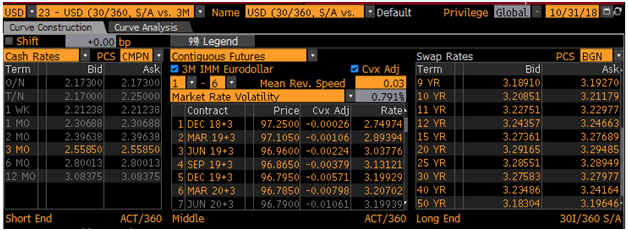
We are going to price a hypothetical bond as at October 31, 2018. We first build a zero coupon curve.  Picture below shows the market rates as at the valuation date.

[caption id="attachment_595" align="aligncenter" width="628"] US swap curve as at Oct 31 2018[/caption]

We utilize the deposit rates (leftmost column) to construct the zero curve up to 12-month maturity. We then use this zero curve to price the following hypothetical fixed rate bond:

Currency: USD

Maturity: 1 year

Payment frequency: semi-annual

Coupon rate: 3%

We use Python [1] to build a bond pricer. Picture below shows the result returned by the Python program. The price is $99.94 (per $100 notional).

derivative pricing in python

Click on the link below to download the python code.


References

[1]  Quantlib Python Cookbook, Balaraman and Ballabio, Leanpub, 2017

Article Source Here: Valuing a Fixed Rate Bond-Derivative Pricing in Python