Parkinson Historical Volatility Calculation – Volatility Analysis in Python

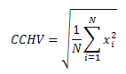
In the previous post, we discussed the close-to-close historical volatility. Recall that the close-to-close historical volatility (CCHV) is calculated as follows,

where x_i are the logarithmic returns calculated based on closing prices, and N is the sample size.

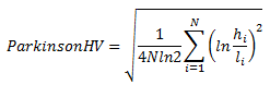
A disadvantage of using the CCHV is that it does not take into account the information about intraday prices. The Parkinson volatility extends the CCHV by incorporating the stock’s daily high and low prices. It is calculated as follow,

where h_i denotes the daily high price, and l_i is the daily low price.

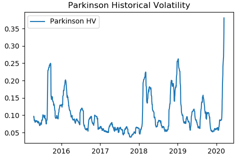
We implemented the above equation in Python. We downloaded SPY data from Yahoo finance and calculated the Parkinson volatility using the Python program. The picture below shows the Parkinson historical volatility of SPY from March 2015 to March 2020.

The Parkinson volatility has the following characteristics [1]

Advantages

• Using daily ranges seems sensible and provides completely separate information from using time-based  sampling such as closing prices

Disadvantages

• It is really only appropriate for measuring the volatility of a GBM process. It cannot handle trends and jumps
• It systematically underestimates volatility.

Follow the link below to download the Python program.

 

References

[1] E. Sinclair, Volatility Trading, John Wiley & Sons, 2008

 

Post Source Here: Parkinson Historical Volatility Calculation – Volatility Analysis in Python

Accounting for Employee Stock Options, Examples and Valuation Methods

International Financial Reporting Standard -2 deals with the recognition, measurement, and disclosure of Employee Stock Options. In this article, we will offer examples of accounting for Employee Stock Options. At the end of this article, we will present methods for valuing Employee Stock Options.

What is an Employee Stock Option?

A company often has the policy to make its employees the shareholders; therefore they offer a certain number of shares to eligible employees as an incentive.

To retain and motivate the workforce and sometimes to comply with the regulatory requirement, the company’s management can opt to issue share options to its employees. The Employee Stock Option plan is not meant to apply to all employees, rather to those who meet certain prescribed criteria.

Employees are normally required to meet the performance as well as service criteria to be eligible for the Employee Stock Option plan. Suppose that the management imposes a service condition of five years and an employee, Mr. A, opted for this option, then after five years of service, he would become eligible to exercise his options. The company often fixes a strike price for the option holders to exercise their rights.

Eligibility of employees

It’s up to the company’s management to decide what criteria they should use when issuing Employee Stock Options, but typically it involves the fulfillment of performance obligation and service period.

Example

Company A has offered 500 share options to each of 5 managers, subject to achievement of their sales targets and continuous services of 5 years with the company. Until these conditions are not fulfilled, the company cannot book expenses for those shares in its accounting books. When the options expire, the employees can choose to settle the transaction either in equity or in cash.

Equity-settled options

In this case, the employees reserve the right to convert their share options into equity by paying only the option exercise price. The employees then become the shareholders of the company.

Cash settled options

In this case, the company offers the employees the option of selling the shares or to get cash equivalent to the market value of those shares.

From the accounting perspective, the company has to make accounting adjustments for both the equity-settled and cash-settled transactions.

How to account for the Employee Stock Options in the financial statement

At the time of offering share options, the company would need to determine the fair value of options or intrinsic value of those options. Then every year after, an expense for compensation shall be debited to employee compensation account and credit entry shall be made in outstanding balance for the compensation plan. The same pattern of entries shall be repeated until the completion of the vesting period. The vesting period is the period after which the employee would be eligible to exercise his/her right to purchase the common stock of the company.

At the end of the vesting period, the employee is offered two options: either to buy common stocks by exercising his/her options, or to get cash equivalent to the number of shares. If an employee chooses to buy shares then the balance in the outstanding account shall be debited and credit shall be made in the capital account as common stocks. If he opts for the cash option, then the outstanding account shall be debited and cash account shall be credited.

How to value Employee Stock Options

Monte Carlo and the Binomial Tree methods are the most common approaches used to price the Employee Stock Options.

Post Source Here: Accounting for Employee Stock Options, Examples and Valuation Methods

Close-to-Close Historical Volatility Calculation – Volatility Analysis in Python

In a previous post, we touched upon a stock’s volatility through its beta. In this post, we are going to discuss historical volatilities of a stock in more details.

Also referred to as statistical volatility, historical volatility gauges the fluctuations of underlying securities by measuring price changes over predetermined periods of time. It is the less prevalent metric compared to implied volatility because it isn't forward-looking.

When there is a rise in historical volatility, a security's price will also move more than normal. At this time, there is an expectation that something will or has changed. If the historical volatility is dropping, on the other hand, it means any uncertainty has been eliminated, so things return to the way they were. Read more

There are various types of historical volatilities such as close to close, Parkinson, Garman-KIass, Yang-Zhang, etc. In this post, we will discuss the close-to-close historical volatility.

The close-to-close historical volatility (CCHV) is calculated as follows,

where x_i are the logarithmic returns calculated based on the stock's closing prices,  and N is the sample size.  In this example, N=22, the average number of trading days in a month.

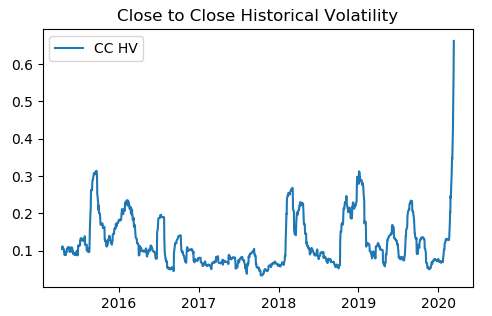
We implemented the above equation in Python. We downloaded SPY data from Yahoo finance and calculated CCHV using the Python program. The picture below shows the close-to-close historical volatility of SPY from March 2015 to March 2020.

It’s observed that the volatility is a mean-reverting process. The CCHV has the following characteristics [1]

Advantages

• It has well-understood sampling properties
• It is easy to correct bias
• It is easy to convert to a form involving typical daily moves

Disadvantages

• It is a very inefficient use of data and converges very slowly

Follow the link below to download the Python program.

 

References

[1] E. Sinclair, Volatility Trading, John Wiley & Sons, 2008

Article Source Here: Close-to-Close Historical Volatility Calculation – Volatility Analysis in Python

What is Stock Beta and How to Calculate Stock Beta in Python

In finance, beta measures a stock's volatility with respect to the overall market. It is used in many areas of financial analysis and investment, for example in the calculation of the Weighted Average Cost of Capital, in the Capital Asset Pricing Model and market-neutral trading.

Beta of an investment is a measure of the risk arising from exposure to general market movements as opposed to idiosyncratic factors.

The market portfolio of all investable assets has a beta of exactly 1. A beta below 1 can indicate either an investment with lower volatility than the market, or a volatile investment whose price movements are not highly correlated with the market. An example of the first is a treasury bill: the price does not fluctuate significantly, so it has a low beta. An example of the second is gold. The price of gold fluctuates significantly, but not in the same direction or at the same time as the market.

A beta greater than 1 generally means that the asset both is volatile and tends to move up and down with the market. An example is a stock in a big technology company. Negative betas are possible for investments that tend to go down when the market goes up, and vice versa. There are few fundamental investments with consistent and significant negative betas, but some derivatives like put options can have large negative betas. Read more

In this post, we present a concrete example of calculating the beta of Facebook, a technology stock. As for the market benchmark, we utilize SPY.

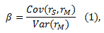
The beta of a financial instrument is calculated as follows,

where

• r_S is the stock return,
• r_M is the market return,
• Cov denotes the return covariance and,
• Var denotes the return variance.

We downloaded 5 years of data from Yahoo Finance and implemented equation (1) in Python.  The picture below shows the result returned by the Python program

It’s observed that the beta of Facebook is 1.19, which means that Facebook is more volatile than the market.

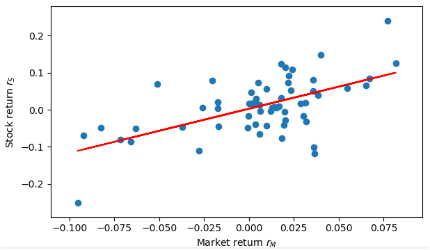
The next picture shows the stock returns regressed against market returns. Note that the slope of the linear regression line equals the beta of the stock.

Follow the link below to download the Python program.

Article Source Here: What is Stock Beta and How to Calculate Stock Beta in Python

Correlation Between the VVIX and VIX indices

The VIX index is an important market indicator that everyone is watching. VVIX, on the other hand, receives less attention. In this post, we are going to take a look at the relationship between the VIX and VVIX indices.

While the VIX index measures the volatility risks, VVIX measures the volatility-of-volatility risks. Its calculation methodology is similar to the VIX’s except that instead of using SPX options it uses VIX options.

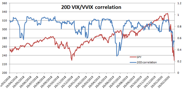
To study the relationship between these 2 indices, we first calculated the rolling 20-days correlation of the VIX and VVIX returns from January 2007 to March 2020. The median value of correlation is 0.807 and 25% quantile is 0.66

The figure below presents the rolling 20-days VIX/VVIX correlation for the last 2 years. We also superimposed SPY on the chart. We observe that the correlation is usually high but there are periods where it decreases significantly. The current period is one of those.

[caption id="attachment_393" align="alignnone" width="628"] Correlation between the VVIX and VIX indices[/caption]

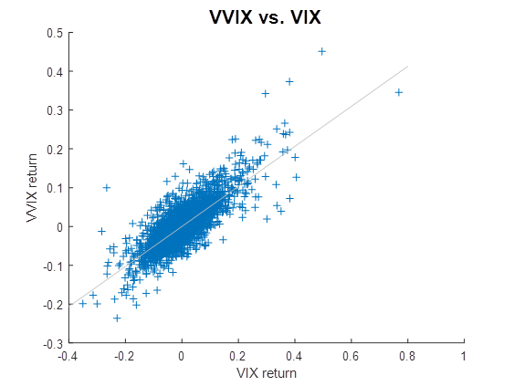
The next figure shows the scatter plot of VVIX returns vs. VIX returns. It’s observed that there is a significant population where VIX and VVIX returns are of opposite signs.  We subsequently calculated the number of instances where VIX and VVIX move in the opposite direction. This indeed happens 22% of the time.

[caption id="attachment_394" align="aligncenter" width="563"] VVIX returns vs. VIX returns[/caption]

Some implications of this study are:

• Although the correlation between VIX and VVIX appears to be high, there is a significant number of instances where VIX and VVIX move in the opposite direction. So it’s fair to say that VVIX follows separate price dynamics which is different from the VIX. In other words, VVIX prices in different risks.
• Long VIX options or SPX back spreads are not always a good hedge for an equity portfolio. The hedge can break down.
• At times it’s cheaper to hedge a long equity portfolio using SPX options; at times it’s cheaper using VIX options.

See More Here: Correlation Between the VVIX and VIX indices

Value At Risk – Financial Risk Management in Python

Value at Risk (VaR) is a tool for measuring a portfolio’s risk.

Value at risk (VaR) is a measure of the risk of loss for investments. It estimates how much a set of investments might lose (with a given probability), given normal market conditions, in a set time period such as a day. ... For a given portfolio, time horizon, and probability p, the p VaR can be defined informally as the maximum possible loss during that time after we exclude all worse outcomes whose combined probability is at most p. This assumes mark-to-market pricing, and no trading in the portfolio.

For example, if a portfolio of stocks has a one-day 5% VaR of $1 million, that means that there is a 0.05 probability that the portfolio will fall in value by more than $1 million over a one-day period if there is no trading. Informally, a loss of $1 million or more on this portfolio is expected on 1 day out of 20 days (because of 5% probability). Read more

There are basically 3 methods for calculating the VaR [1]

1. Historical simulation
2. Variance-covariance approach
3. Monte Carlo simulation

In this post, we implement the 3^rd method, i.e. the Monte Carlo simulation, in Python.  More details of the methodology can be found in Ref [1].

The simulation parameters are as follows,

• Portfolio value: $1 Million
• Confidence interval: 95%
• Time horizon: 1 day
• Underlying: SPY

We utilize 5-years daily data of SPY retrieved from Yahoo Finance. The picture below shows the VaR retuned by the Python program.

Note that the method presented in this post is suitable for calculating the VaR in a normal market condition. More advanced approaches such as Expected Tail Loss have been developed that can better take into account the tail risk.

Follow the link below to download the Python program.

References

[1] Hull, John C. (2003). Options, Futures, and Other Derivatives. Prentice-Hall

Article Source Here: Value At Risk – Financial Risk Management in Python

Another Misuse of Financial Derivatives

Just like any financial derivatives that were initially designed for risk management purposes, interest rate swaps are an effective tool for managing and transferring interest rate risks as long as those risks are well understood.  But as banks and financial institutions are constantly trying to invent new financial products to sell to their consumers, sometimes the risks of those products are not well understood and disclosed.

This is what happened with the interest rate swap market in New Zealand where banks sold interest rate swaps to farmers in order for them to hedge the fluctuation in the mortgage rates.  However, the banks only emphasized the advantages of the interest rate swaps, and they did not discuss the potential downside in detail.

Swaps are enormously complicated and risky financial derivatives. They are used - mostly by big businesses or international dealing rooms - to hedge against interest rate moves.

But in the period 2005-2008, New Zealand banks aggressively sold swaps to farmers as a supposedly less risky alternative to fixed interest loans, and a way for farmers to protect themselves from hikes in their mortgage repayments if interest rates went up.

When the financial crisis hit, and the interest rates went down, farmers started losing money. Many were forced to sell their farms, and some of them committed suicide.

Walker estimates up to 2000 New Zealand farmers lost up to $1 billion on swaps. They lost farms they had inherited from their fathers and planned to pass onto their children. Too many committed suicide. Walker spent the three years following the Farmers Weekly survey doggedly researching banks' sales of swaps to New Zealand farmers. And then she went to see the regulators.  Read more

The problem is not in the financial derivative itself, but it is that the risks were not well understood and explained to the customers.

Banks will be asking what are the lessons, what do we need to change to make sure going forward we don't have this happen with a different product. It's not so much just about the swaps but how do we make this not happen in the future.

Article Source Here: Another Misuse of Financial Derivatives

Accounting for Convertible Debt

Convertible debt is a type of loan that can be converted back to stock after some specified future date. When making an investment in convertible debt, both the issuer and investor are clear that there is a possibility of debt being converted into stock in the future. International Account Standard 32 deals with accounting for convertible debt.

A convertible debt instrument is an alternative financing solution, normally used by companies to finance their operation or working capital. The peculiar thing about this arrangement is that both parties can be on the same page regarding an eventual conversion of convertible debt into common stock of the company. In other words, both the issuer and the holder can convert the debt into equity at a future date. However, the former (i.e. the forced conversion) is rare, while the latter (conversion by the holder) is more common.

Sometimes, it is not easy for the company to issue convertible debt because the shareholder may oppose this management decision. This is due to the fact that upon conversion of the debt to equity, the shareholders’ stock values will decline because of the share dilution. Therefore management needs to pursue by performing a cost-benefit analysis as to why the issuance of convertible debt is beneficial to the company and its shareholders at the same time.

An example of a convertible debt

Normally, the company issues the bond at par, but sometimes it can offer a discount to investors in convertible debts as an incentive. For example, Mr. A purchased a convertible bond on January 01, 2020, for $500,000 at $500 each, whereas the par value of the bond is $550. Why has the company offered a discount on the issuance of the bond?  It is because investors will be likely to convert their debts into equities.

Why offering a discount?

Debt is senior to equity in terms of payback at times of liquidation. So if an investor is willing to forgo his debt right for equity, then obviously the company has to offer some incentive in order to keep its investment.

Moving forward in the above-mentioned example, if the maturity of the bond is December 31, 2024, this means that after 5 years, the investor can convert and the company can reduce its debts leverage and issue its stocks in place.

Why is issuing a convertible bond good for the company?

A company at times is in need of financing, but they don’t want to increase their debt leverage, therefore they offer a discount to investors for investing in their convertible debt instruments. Once the investment has been made, the company can save itself from a debt burden.

Why is purchasing a convertible bond good for investors?

Often times it is worthwhile to invest in a company’s stock but for some reason, the investor does not want to invest in equity immediately. Therefore a better way is to go for convertible debt and then convert it into equity at a future date. This way, the investor will be in the position of a shareholder. In addition, as discussed above, the investor can be offered a discount as an incentive for investing in convertible debt.

How to account for the convertible debt:

As both the company and investors have the same understanding that after a defined period of time they can convert the debt into common stocks, therefore as per IAS-32, when accounting for the convertible debt, the company has to recognize the issuance of convertible debts as a compound instrument.

Every year the interests accrued on the debt portion of the convertible debt shall be recognized in the profit and loss statement, and at the maturity of that instrument, all the loan shall be converted into equity at par and will be recognized in the capital of the company.

Post Source Here: Accounting for Convertible Debt

Valuing European Options Using Monte Carlo Simulation-Derivative Pricing in Python

In a previous post, we presented a methodology for pricing European options using a closed-form formula. In this installment, we price these options using a numerical method. Specifically, we will use Monte Carlo simulation.

Recall that,

• A call option gives the buyer the right, but not the obligation to buy an agreed quantity of the underlying from the seller at a future time for a given price. The payoff of the call option at expiration is max(S_T-K,0),
• A put option gives the buyer the right, but not the obligation to sell an agreed quantity of the underlying to the seller at a future time for a given price. The payoff of the put option at expiration is max(K -S_T,0),

where S_T  denotes the stock price at expiration and K is the strike price.

To price these options, we first simulate the price paths using the following Stochastic Differential Equation:

where

• S_t is the stock price at time t,
• σ denotes the stock volatility,
• µ is the drift which equals the risk-free rate, and
• dW_t represents the standard normal random variable.

The simulation is carried out until the options’ maturity. We then apply the terminal payoff functions and calculate the mean values of all the payoffs. Finally, we discount the mean values to the present and thus obtain the option values.  For a more detailed presentation of the Monte Carlo method, see Reference [1].

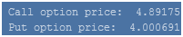
The picture below shows the call and put option prices using 100000 simulations. All other parameters are the same as in the previous post.

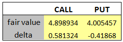
We compare the above results to the ones obtained by using a third-party software and notice that they are in good agreement.

In the next installment, we will present a methodology for pricing American options using Monte Carlo simulation.

References

[1] Glasserman, Paul; Monte Carlo Methods in Financial Engineering, Springer; 2003

 

Follow the link below to download the Python program.

Originally Published Here: Valuing European Options Using Monte Carlo Simulation-Derivative Pricing in Python

Black-Scholes-Merton Option Pricing Model-Derivative Pricing in Python

The Black-Scholes-Merton model is one of the earliest option pricing models that was developed in the late 1960s and published in 1973 [1,2]. The most important concept behind the model is the dynamic hedging of an option portfolio in order to eliminate the market risk. First, a delta-neutral portfolio is constructed, and then it is adjusted to stay delta neutral as the market fluctuates. Finally, we arrive at a Partial-Differential Equation for the value of the option.

where

• V denotes the option value at time t,
• S  is the stock price,
• r is the risk-free interest rate and,
• σ is the stock volatility.

This equation is also called a diffusion equation, and it has closed-form solutions for European call and put options. For a detailed derivation and analytical formula, see Reference [3].

In this post, we focus on the implementation of the Black-Scholes-Merton option pricing model in Python. Closed-form formula for European call and put are implemented in a Python code. The picture below shows the prices of the call and  put options for the following market parameters:

• Stock price: $45
• Strike price: $45
• Time to maturity: 1 year
• Risk-free rate: 2%
• Volatility: 25%

We compare the above results to the ones obtained by using third-party software and notice that they are in good agreement.

In the next installment, we will price these options using Monte Carlo simulation.

References:

[1] Black, Fischer; Myron Scholes (1973). The Pricing of Options and Corporate Liabilities. Journal of Political Economy. 81 (3): 637–654

[2] Merton, Robert C. (1973). Theory of Rational Option Pricing. Bell Journal of Economics and Management Science.

[3] Hull, John C. (2003). Options, Futures, and Other Derivatives. Prentice Hall

 

Follow the link below to download the Python program.

Originally Published Here: Black-Scholes-Merton Option Pricing Model-Derivative Pricing in Python