Accounting for Stock Warrants

A stock warrant is a contract between a company and investors, which gives them the right to purchase newly issued shares of a stock at a set price for a set period of time. The company directly issues the new stock instead of using issued stock. However, investors that get a stock warrant do not have a legal right to the ownership of stock, but only a right to purchase it in the future. Similarly, for the company, a stock warrant does not lock in investors to buy the stock. They still have a choice of not exercising the right.

Since the warrant sets the price of the newly issued stock, it can be beneficial to the investors. Especially when the price of the company's stock rises in the stock market, investors can profit from the lower price of stocks offered to them through warrants. Similarly, the market price of the stock of a company will not affect the price of the warrant, as the company issues the new stocks, and the price is preset.

There are many different types of stock warrants that companies may put into use. The two main types of stock warrants are put and call warrants. A put warrant limits the amount of equity that the investor can sell back to the company at a given price. A call warrant, on the other hand, guarantees the investor’s right to purchase a predetermined number of shares at a predetermined price. There are also other types of warrants such as covered, naked, traditional, and wedded warrants. These are classified based on the degree of risk and value of the warrant.

Accounting for Stock Warrants

When it comes to accounting for stock warrants, the company issuing them must ensure two things. First, the company must recognize the fair value of the equity instrument issued or the fair value of the consideration received, based on whichever is reliably measurable. Second, the company must recognize the asset or expense related to the goods or services at the same time.

If the option to exercise the stock warrant expires, the company cannot reverse the related expense or asset recognized. Furthermore, if a company receives warrants in exchange for products or services, it can recognize revenues normally, as they would under the accounting standard related to revenue.

Once the company determines the fair value of the stock warrant, the company can use the following accounting treatment to account for the transaction.

Dr Expense/Asset

Cr Stock warrants

When the investor exercises the option to avail the stock warrants, the company can use the following accounting treatment to convert the stock warrant balance into equity.

Dr Stock warrants

Cr Share capital

Cr Share premium

The value of the share capital and share premium will depend on the original fair value measurement of the company.

Valuation of Stock Warrants

A warrant can be valued using the binomial tree approach. Dilution needs to be taken into consideration. Basically, the valuation proceeds as follows,

1. Build a tree for the underlying stock
2. Calculate the warrant value at each end node of the tree.
3. Move on to the previous time step and calculate the warrant value at each node on this time slice using the warrant values at the precedent nodes.
4. After the warrant value is calculated at a node, check whether early exercise is allowed and optimal. The warrant price at this node is then the greater of this value and the payoff of the early exercise.
5. Continue in this manner until the warrant is valued at all nodes of the tree.
6. The value at the root node of the tree is the price of the warrant at the valuation date.

Conclusion

A stock warrant gives investors the right to purchase newly issued shares of a company at a set price within a set period of time. The accounting treatment of stock warrants requires the company to determine the fair value of the stock warrant at the date of measurement. When the investor exercises the right to buy shares, the company must convert the stock warrant's balance to equity.

Article Source Here: Accounting for Stock Warrants

Accounting For Stock Options

A stock option is a contract between a company and its investors that gives them the right to buy or sell underlying stocks at a preset price within a specific time period. Just like ordinary stocks of a company, its stock options are also available for trade on stock exchanges. These options may come at a higher or lower price depending on when they were listed originally. In addition to stock options traded on the stock market, companies may also issue stock options to their employees. Employee stock options allow the employees of a company the right to purchase shares at a predetermined rate and period of time.

The price of a stock option is directly related to the price of the underlying stock. If the price of the stock fluctuates, the option will also change accordingly. Similarly, stock options can have other characteristics too. Stock options come in two types, calls and puts. A call option allows the investor to buy shares at a set price within a predetermined time. On the other hand, a put option allows the investor to sell shares at a predetermined rate within a predetermined time.

Stock options also have a strike price, which is the price at which investors can exercise the stock option. Likewise, stock options also have a premium, which represents the profit for the company selling the option. The premium depends on the price the buyer pays for the option. Usually, it will also depend on the price of the underlying stock in the market.

Stock options also have a grant date, a vesting date and an exercise date. The grant date is the date on which the company grants these options. The vesting date is the date on which the buyer obtains the right to exercise the option. The period between the grant date and the vesting date is known as the vesting period. Lastly, the exercise date is the date on which the buyer exercises the option and buys the underlying shares.

Accounting Treatment

The accounting treatment for stock options depends on the different dates related to them. First of all, when a company grants stock options to investors or employees, it does not require any accounting treatment. That is because, at the grant date, the stock options do not have any effect on the company.

As mentioned above, the period after the grant date but before vesting date is known as the vesting period. The vesting period of a stock option may span over several years. Therefore, at the end of each accounting period, the company must estimate the fair value of the number of equity instruments expected to vest through stock options. Once the company determines the fair value, it can expense it out as follows:

Dr Compensation Expense/Asset

Cr Equity (Stock options)

On the exercise date, when the buyer buys the shares, the company will record the payment as follows.

Dr Cash

Dr Equity (Stock options)

Cr Equity (Share Capital)

Cr Equity (Share premium)

In the above accounting treatment, the company reverses the equity recognized as stock options and recognizes share capital and share premium, if any.

Valuing Stock Options

There are different models for valuing options. The earliest model is called the Black-Scholes option pricing model which provides an analytical, closed-form formula for valuing a European option.

Binomial option model is used to value American style options. The model relies on the assumption that for the next time period, a stock can move up, or down with certain probabilities. The major advantage of the binomial model is that it’s relatively simple.

An option can also be valued using Monte Carlo simulation. The simulation is carried out until the options’ maturity. We then apply the terminal payoff functions and calculate the mean values of all the payoffs. Finally, we discount the mean values to the present and thus obtain the option value.

Conclusion

A stock option is an instrument that a company offers to its investors, which gives them the right to buy or sell the stocks of the company at a set price within a specific period of time. The company may also offer stock options to its employees. The accounting treatment of stock options depends on the vesting period and exercise date of the option.

Originally Published Here: Accounting For Stock Options

Implied Volatility of Options-Volatility Analysis in Python

Volatility measures market expectations regarding how the price of an underlying asset is expected to move in the future. There are two types of volatility: historical volatility and implied volatility. In a series of previous posts, we presented methods and provided Python programs for calculating historical volatilities. In this post, we are going to discuss implied volatility and provide a concrete example of implied volatility calculation in Python.

In financial mathematics, the implied volatility (IV) of an option contract is that value of the volatility of the underlying instrument which, when input in an option pricing model (such as Black–Scholes), will return a theoretical value equal to the current market price of said option. A non-option financial instrument that has embedded optionality, such as an interest rate cap, can also have an implied volatility. Implied volatility, a forward-looking and subjective measure, differs from historical volatility because the latter is calculated from known past returns of a security. To understand where implied volatility stands in terms of the underlying, implied volatility rank is used to understand its implied volatility from a one-year high and low IV. Read more

Since there is no analytical formula for calculating the implied volatility of an option, we must use numerical root-finding techniques. While there are many techniques for finding roots, two of the most commonly used are Newton's method and Brent's method.  More details about these methods can be found in Reference [1].

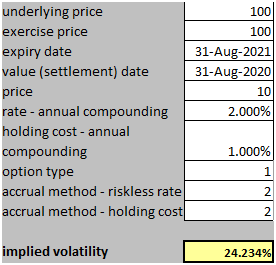
In this post, we utilize a Python program to calculate the implied volatility of a European call option. The parameters of the option are as follows.

Valuation date: August 31, 2020

Expiry: August 31, 2021

Option type: Call

Exercise type: European

Option price: 10

Strike: 100

Underlying asset price: 100

Risk-free rate: 2%

Dividend yield: 1%

The picture below shows the implied volatility calculated by the Python program

We note that the implied volatility calculated by the Python program agrees well with the result obtained by using a third-party program as shown below.

Click on the link below to download the Python program.

References

[1] William H. Press, Saul A. Teukolsky, William T. Vetterling , Brian P. Flannery, Numerical Recipes 3rd Edition: The Art of Scientific Computing, Cambridge University Press, 3rd Edition, 2007.

Post Source Here: Implied Volatility of Options-Volatility Analysis in Python

Are AI-Powered Hedge Funds Outperforming?

Last month, institutionalinvestor.com reported that AI-powered hedge funds outperformed their peers,

Hedge funds with artificial intelligence capabilities showed a huge competitive edge over investors that didn’t use AI, new research indicates.

AI-led hedge funds produced cumulative returns of 34 percent in the three years through May, a report Tuesday from consulting and research firm Cerulli shows. That compares with a 12 percent gain for the global hedge fund industry over the same period. Read more

However, things are not so bright under the surface. It was recently reported that one of the largest AI hedge funds is underperforming,

Voleon Group, one of the world’s biggest and best-performing artificial intelligence hedge funds, has suffered large losses after being hit by choppy markets, making it one of a number of computer-driven fund managers to struggle this year

...like many computer-driven funds, Voleon was caught out by this year’s market turmoil. That had left the Investors fund down by double digits earlier this year, and the Institutional Strategies fund down single digits, say people familiar with its returns.

Voleon is unusual in that, while many quantitative fund firms use a small element of machine learning in their investment process, very few focus solely on this approach. Machine learning involves letting algorithms learn and extrapolate rules from the data, rather than a human setting the rules an algorithm should follow. The firm trades a strategy known as statistical arbitrage, which involves betting that short-term discrepancies in prices will revert to a mean. Read more

Article Source Here: Are AI-Powered Hedge Funds Outperforming?

How to Calculate Stock Beta in Excel-Replicating Yahoo Stock Beta

In a previous post, we presented a method for calculating a stock beta and implemented it in Python. In this follow-up post, we are going to implement the calculation in Excel. We continue to use Facebook as an example. Recall that,

In finance, the beta (market beta or beta coefficient) is a measure of how an individual asset moves (on average) when the overall stock market increases or decreases. As such, beta is a useful measure of the contribution of an individual asset to the risk of the market portfolio when it is added in small quantity. Thus, beta is referred to as an asset's non-diversifiable risk, its systematic risk, market risk, or hedge ratio. Beta is not a measure of idiosyncratic risk. Read more

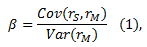
We utilize the following equation to calculate the stock beta,

where

• r_S is the stock return,
• r_M is the market return,
• Cov denotes the return covariance and,
• Var denotes the return variance.

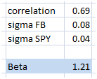
We downloaded 5 years of monthly Facebook data from Yahoo Finance. We implemented the above equation in Excel and obtained a beta of 1.21

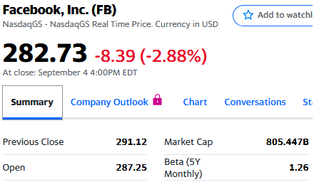
The picture below shows Facebook beta calculated by Yahoo Finance. It is 1.26. Our result agrees well with Yahoo’s result, although there is a small difference.

Click on the link below to download the Excel workbook.

Also, let us know what you think where the difference comes from.

Article Source Here: How to Calculate Stock Beta in Excel-Replicating Yahoo Stock Beta

Valuation of Executive Stock Options Using a Closed-Form Formula

Executive stock options usually have complex payoffs. To price them, we often use the binomial tree method or Monte Carlo simulations.

... a lattice model can be designed to accommodate dynamic assumptions of expected volatility and dividends over the option's contractual term, and estimates of expected option exercise patterns during the option's contractual term, including the effect of blackout periods. Therefore, the design of a lattice model more fully reflects the substantive characteristics of a particular employee share option or similar instrument. Nevertheless, both a lattice model and the Black–Scholes–Merton formula, as well as other valuation techniques that meet the requirements ... can provide a fair value estimate that is consistent with the measurement objective and fair-value-based method. Read more

Recently, Hsiao et al. [1] derived a close-form solution to a particular class of executive stock options.

This study derives a closed-form approximate solution for Bermudan reset executive stock options with cash dividends. The complicated payoff characteristic of this exotic option is caused by its particular stylistic features, including the reset mechanism, cash dividends, early exercises, and increasing volatilities. Using the integral representation method, a closed-form approximate solution was successfully derived. Moreover, this study discusses how specific critical factors affect executive stock option values and arrives at some interesting results by way of a numerical calibration.

 

References

[1]  Y.L. Hsiao, L.L. Chen, C.J. Ting,  The Valuation of Executive Stock Option Using the Integral Representation Method, Journal of Mathematical Finance, 2020, 10, 431-447

Article Source Here: Valuation of Executive Stock Options Using a Closed-Form Formula

Valuation of Callable Puttable Bonds-Derivative Pricing in Python

In a previous post, we presented a method for pricing a fixed-rate bond. In this post, we are going to discuss valuation of a callable bond.

A callable bond (also called redeemable bond) is a type of bond (debt security) that allows the issuer of the bond to retain the privilege of redeeming the bond at some point before the bond reaches its date of maturity. In other words, on the call date(s), the issuer has the right, but not the obligation, to buy back the bonds from the bond holders at a defined call price. Technically speaking, the bonds are not really bought and held by the issuer but are instead cancelled immediately.

The call price will usually exceed the par or issue price. In certain cases, mainly in the high-yield debt market, there can be a substantial call premium.

Thus, the issuer has an option which it pays for by offering a higher coupon rate. If interest rates in the market have gone down by the time of the call date, the issuer will be able to refinance its debt at a cheaper level and so will be incentivized to call the bonds it originally issued. Another way to look at this interplay is that, as interest rates go down, the present values of the bonds go up; therefore, it is advantageous to buy the bonds back at par value. Read more

Valuation of a callable bond requires a short-rate model. The valuation steps are as follows,

1. Calibrate the short-rate model using market data
2. Build an interest-rate tree
3. Price the bond

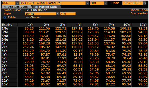
[caption id="attachment_991" align="aligncenter" width="520"] Swaption volatilities. Source: Bloomberg[/caption]

We are going to present a concrete example of pricing a callable bond. The parameters of a hypothetical callable bond are as follows,

Valuation date: June 30, 2020

Issue date: September 30, 2019

Maturity: 5 years

Coupon: 2.5%

Call strike: 100

Call period: September 30, 2019 to maturity

We chose the Hull-White model to describe the interest rate dynamics.  This model is widely used in practice because it allows for the model to fit the term structure of interest rates. We utilize the method presented in Reference 1 in order to calibrate the model parameters to the market data. Specifically, we use swaption volatilities in the calibration and obtain σ=0.676% and α=0.127% as at the valuation date.

We then use a Python program to build a trinomial tree for the risk-free rates following the procedure detailed in References 2 and 3. After a trinomial interest-rate tree is built, the valuation of the callable bond proceeds as follows.

Let’s define the following terms with respect to a node (i,j) :

• i: means that on the node (i,∙) the date is defined by i×dt where dt is the length of the time-step.
• j: means the position (up/medium/down) of the tree,
• C (i,j): call price at node (i,j),
• P (i,j): put price at node (i,j) ,
• R (i,j): the projected risk-free rates at nodes (i,j) which are modeled using the Hull-White interest rate dynamics,
• V(i,j): continuation value of the bond at node (i,j) which is calculated as the expectation value of the continuation values of the next three possible nodes originating from (i,j) discounted by one period using the projected rates R(i,j).

The values of the bond at the terminal nodes N, where N=T/dt, and T is the time to maturity, is set to the notional at maturity (Notional_N) plus the interest payment at that time (interest_N), i.e.

V(N,∙)=Notional_N+ interest_N,

We then move back to the previous time step and calculate the bond continuation value at each node on this time slice using the continuation values at its precedent nodes and add any interest payment that occurs between the two time steps.

If the bond is callable at time i×dt, then the value of the bond is calculated as,

V(i,j)=min( V(i,j),C(i,j))

i.e. the issuer will exercise the call if the call value is smaller than the continuation value; that is, the position of the issuer can be improved by calling the bond.

Similarly, if the bond is puttable at time i×dt, then the value of the bond is calculated as,

V(i,j)=max( V(i,j),P(i,j))

i.e. the bond holder will exercise the put if the put value is greater than the continuation value.

The above procedure is repeated until we reach the root of the tree. The value of the callable/puttable bond at the valuation date is the continuation value at time zero.

The picture below shows the price of the hypothetical callable bond calculated by the Python program.

Click on the link below to download the Python program.

References

[1] Hull, J. C. (2018), Options, Futures and Other Derivatives (10th Ed.), Prentice-Hall

[2]  Hull, J. C. and White, A. 1994, Numerical Procedures for Implementing Term Structure Models I: Single Factor Models, Journal of Derivatives

[3]  Hull, J. C. and White, A. 1996, Using Hull-White Interest-Rate Trees, Journal of Derivatives

Post Source Here: Valuation of Callable Puttable Bonds-Derivative Pricing in Python

Short Volatility Funds Lost Money During The Pandemic

With a sudden increase in volatility during the pandemic, many volatility funds lost money.

Many funds were struck because they adopted a strategy known as shorting volatility — betting that it will fall or remain low. Such funds sell derivative protection such as put options, which give the buyer the right to sell at a pre-determined price. They earn money by effectively writing market insurance, hoping that volatility — which helps determine options prices — will remain low and the options will expire worthless.

Many investors have been lured into taking this approach over the past decade by years of gently rising markets and mild market moves, fuelled by trillions of dollars of central bank stimulus, which have helped such funds make money. Read more

One of the most notable cases was the Alberta Investment Management Corporation’s loss of $3 billion.

The Alberta Investment Management Corp. — which manages pension assets, sovereign wealth, and other public money — lost billions of dollars on wrong-way volatility trades when markets crashed earlier this year, and then shut down the strategies, according to informed sources.

The now-defunct volatility-trading program cost pensioners and Albertans about $3 billion, the sources said. That’s on top of substantial, first-quarter losses to portfolio value that nearly all public funds are dealing with amid the coronavirus crisis. Read more

 

Originally Published Here: Short Volatility Funds Lost Money During The Pandemic

Banks Hold Many Illiquid Assets

The trend in the increased holding of risky assets continues. Because of Covid-19, the big banks now hold more illiquid, opaque assets than before.

Lenders including Barclays Plc, Citigroup Inc., BNP Paribas SA and Societe Generale SA reported a surge of more than 20% in their most opaque assets during the chaotic first half of 2020, Bloomberg calculations show. The banks are now sitting on hard-to-value trades that they say are worth about $250 billion, including categories that gained notoriety during the financial crisis, such as complex debt securities.

These assets are hard to value, and they can cause a financial crisis like the one we had in 2008.

There’s little market data for Level 3 assets -- which include distressed debt, some mortgage-backed bonds, high-risk loans and derivatives linked to everything from interest rates to corporate debt -- so banks get to value them based on historical trends and their own risk assumptions. Read more

Originally Published Here: Banks Hold Many Illiquid Assets

Quantitative Trading

If you’re looking to set up your own algorithmic trading business, quantitative trading is a market you can consider. Many independent investors are exploring the market, learning to generate data, and execute it.

In the past, quantitative trading used to be the business of hedge funds and other financial institutions involving huge sales of shares. The shares in this business run in many hundred thousands, together with the securities. Working for a hedge fund may be the reason you learn about the quantitative trading system.

What is quantitative trading?

Quantitative trading involves using quantitative analysis to identify points with a profitable trade where you can buy assets. This is a branch of quantitative finance. To find an opportunity for trading, a trader has to compute a set of mathematical data in order to determine a market is most likely profitably within a period.

The type of asset involved in a single quantitative trade and the type of research used in the analysis will be the trader’s sole choice. The process of developing a workable trading strategy requires careful study and testing to ascertain the loops in the system before the execution.

Heavy mathematical modeling and computation form the basis of quantitative analysis trading. To keep up with these computations, a trader has to be versed in a relevant computer program. Some of these programs include MATLAB, Python, R, C/C++, network latency optimization, etc.

Breakdown of Quantitative Trading

In quantitative trading, your business is to use the mathematical models you generate to learn the possibility of getting a certain outcome. The only possible way to achieve this in quantitative finance is by using programming and statistics. Your interest is in the volume and price of a trade, not in the strength of the brand.

Therefore, assume that the stock of a certain business rises in volume, which also affects its pricing. You then work out a program targeted at identifying how this pattern occurs in the history of the business. How does this kind of rise affect the market value of this business?

Let’s say the result of your research says the business has experienced a 90% growth from this type of rise over the years. It means that there's a 90% chance for such growth in the future.

Who does Quantitative Trading?

People who have a background in financial modeling, math, or engineering are more likely to excel in quantitative analysis, and by extension, quantitative trading. Added to these skills, these individuals need a strong understanding and ability to handle any of the programming software that includes Python, R, and C/C++, plus APIs (application programming interfaces).

Some of the added skills that a funds company will need a person to have included being able to create automated data and mine data. These are the same skills an individual trader needs. However, you should also have a proficiency in understanding kurtosis, VaR (Value at Risk), and conditional probability.

Quantitative trading involves mathematical computations in all of its entirety. This feature is what distinguishes it from the traditional investment platform where you consider brand behavior.

A trait that you’ll find among traders is that they may decide to customize an existing strategy that is proven as successful, in addition to building their own. They go ahead to create programs that help them identify the opportunities in a strategy, thereby creating time to research more strategies.

A part of the job of quantitative traders is the high-frequency trading (HFT). In HFT, they work on many positions in the short term, opening and closing with the help of programming.

This strategy is not for every fund group or trader. In some cases, the trader uses a model to find out trades that are larger and less frequent as part of their strategy for the long-term.

Traders who use HFT need computer programs for this technique because it involves so many short transactions that should be identified and executed at once. A programming strategy would be more efficient than human analysis to avoid time lapse and loss.

Major components of Quantitative Trading

Singling out opportunities and executing them are the basics of every quantitative trading system. Every system is unique in the way it identifies positions and executes. But, the components are integrated across the board.

They include:

• Identifying the Strategy
• Backtesting it
• System of Execution
• Risk Management

Here’s a breakdown of these concepts.

Identifying the Strategy

Every process of quantitative trading starts with research. Research helps you to find your strategy. You can analyze this strategy by fitting it into your existing portfolio, to check if it aligns with your other strategies. Further, obtain all data necessary to test your strategy while optimizing it for lower risks and more returns.

As an individual trader, factor in the costs involved, including your capital and the effect of these transactions.

Public sources can be a good place to find strategies that are profitable. These sources include trade journals, academic publications, and quantitative finance blogs. The details they offer vary as well.

Public source strategies do not include the parameters and methods of tuning. If you are able to find a suitable pattern for optimizing them, these can become highly profitable strategies.

A strategy can have Low-frequency trading (LFT), high-frequency trading HFT), and Ultra-high frequency trading (UHFT). These frequencies refer to how long a strategy will hold an asset. LFT will stay longer than one trading day; HFT will hold intraday and UHFT will hold for milliseconds and seconds.

With your strategy set up, the next thing is to backtest it, to know how profitable it is.

Backtesting your strategy

In backtesting, you apply the strategy you picked to both historical and out-of-sample data to prove that it is profitable. Your result tells you what to expect of the strategy in a real trade, even though it doesn’t always translate exactly.

While backtesting, you’ll meet several biases; you’ll need to consider them diligently before eliminating them. The biases will include look-ahead bias, data-snooping bias, and survivorship bias.

Also, look out for how clean and available historical data is, which includes providing a backtesting platform that is robust and costs that are realistic.

After identifying a strategy, get the historical data since this will help you with testing and refinement. Here are some issues that concern using a historical set of data.

Cleanliness/Accuracy

Does the data contain any error? In some cases, it’s easy to pick out errors. Other times, it’s well-hidden in plain sight. If possible, have a team of providers who weigh their data with each other to identify biases.

Survivorship bias

Does the data contain delisted or bankrupt stocks? Are the assets still trading?

Survivorship bias is a feature you look out for in a cheap set of data. You want to know if the assets are in a trade or not. Trades that have left the market or bankrupt stocks will not perform in real life.

Besides, cheap data will often perform better during backtesting than they would in the real world.

Corporate actions

What are the dividend adjustments and stock splits in the trade? That is, activities of the company that take away from the price returns.

In all cases, movements will create a step-function change in the raw price of the company. This change does not form part of the price returns when you’re calculating. In fact, you should carry out back adjustments when you make these changes. You want to avoid confusing a stock split with actual returns adjustments.

When you’ve established your history data set, you need a software platform that can be either of a dedicated backtest software, a complete custom implementation using a programming language, or a numerical platform.

To measure the performance of your strategies, you’ll need to know the maximum drawdown and the Sharpe Ratio. In maximum drawdown, you’re measuring the equity curve drop from peak to trough in a specific period, as a percentage.

In Sharpe Ratio, you’re taking the average of the excess returns and dividing it by their standard deviation. This excess return is measured against the expected benchmark for the strategy’s return.

Done with backtesting, you can then execute.

System of Execution

With the list of trades your strategy has generated, you can build a manual execution system or an automated system. In a manual system, your business is to keep your broker on a call while you place your trades. Otherwise, build a semi-automated or fully-automated system for your execution.

An LFT strategy will thrive on manual or semi-automated systems while HFT strategies are best suited for fully-automated systems. Automated systems help you create extra time to look for more strategies and run them.

3 factors you should consider in creating your execution system include your broker’s interface, how to minimize transaction costs and performance divergence from backtested performance.

Individual traders will often handle their execution themselves while established hedge funds will have their dedicated executor.

In executing, you also need to minimize the cost of transactions which includes commissions, slippage, and spread. The brokerage charges commissions; slippage tells the difference in the price of your order and your initial estimate, while the spread is the gap in the bid/ask price of the security you’re trading. Spread, however, is not a constant factor.

Transaction costs, in itself, can be the shift from a very unprofitable strategy to a highly profitable strategy. These costs can barely be detected in a backtest, which is why you need to be critical about analyzing your transaction costs.

About divergence of strategy from backtested performance, some bugs and invisible trading strategies may only emerge in life transactions. Some of them include a new regulatory environment, macroeconomic phenomena, and change in investor sentiment. All these are in addition to life-ahead, data snooping, and survivorship biases.

Risk Management

Risk management includes your ability to work around the list of biases mentioned before. It also includes the risk of technology (like a dysfunctional server) and brokerage bankruptcy. Think of anything that can impact the trading system; it’s a risk you should manage.

Portfolio theory (i.e. optimal capital allocation) is part of the risk management system. It’s about deciding how to allocate funds to the various strategies and the trades that lie within each strategy. It’s a complex system that requires great thought and diligent execution.

Your personal disposition could also be a threat to your trades. It’ll determine how fast you are with making decisions, your ability to dispassionately make a good decision and to cancel out the greed in your trades.

Pros and Cons of Quantitative Trading

The pros and cons associated with this business is embedded in the transactional process and the returns from it. They are as follows:

Pros

• Quantitative Trading helps you determine how profitable a system before executing a trade
• You can arrive at a less flawed decision through monitoring and analysis before the system is overwhelmed with data
• Computers are efficient in automated monitoring and analysis, therefore enhancing the rate of decision making
• Access to a large market and extensive data points list
• Less emotional involvement since AI handles a good part of the decision making system

Cons

• Ability to remain as dynamic as the financial market system.
• Strategies are often momentarily profitable. Many do not survive changes in the market condition

Conclusion

Quantitative trading is a model that uses mathematical computation to determine existing opportunities. This requires quantitative traders to have an extensive background in mathematics, statistics, programming, and related fields. Creating an effective quantitative trading system requires 4 components including strategy, backtesting, execution, and risk management.

A good majority of quantitative traders work for established systems such as investment firms and hedge funds. However, individuals are beginning to start their own quantitative trading and require more computational skills since they have to manage the system alone.

 

Quantitative Volatility Trading

In this part, we will look at volatility trading from the quantitative perspective.

We first need to estimate the current volatility

Close-to-Close Historical Volatility

The Close-to-Close Historical Volatility has the following characteristics [1]

Advantages

• It has well-understood sampling properties
• It is easy to correct bias
• It is easy to convert to a form involving typical daily moves

Disadvantages

• It is a very inefficient use of data and converges very slowly

Parkinson Historical Volatility

The Parkinson volatility has the following characteristics

Advantages

• Using daily ranges seems sensible and provides completely separate information from using time-based sampling such as closing prices

Disadvantages

• It is really only appropriate for measuring the volatility of a GBM process. It cannot handle trends and jumps
• It systematically underestimates volatility.

Garman-Klass Historical Volatility

The Garman-Klass volatility estimator has the following characteristics

Advantages

• It is up to eight times more efficient than the close-to-close estimator
• It makes the best use of the commonly available price information

Disadvantages

• It is even more biased than the Parkinson estimator

Garman-Klass-Yang-Zhang Historical Volatility

We note that the Garman-Klass-Yang-Zhang  volatility estimator takes into account overnight jumps but not the trend, i.e. it assumes that the underlying asset follows a GBM process with zero drift. Therefore the GKYZ volatility estimator tends to overestimate the volatility when the drift is different from zero. However, for a GBM process, this estimator is eight times more efficient than the close-to-close volatility estimator.

We now present a volatility trading system on a volatility ETF.

The trading rules are as follows

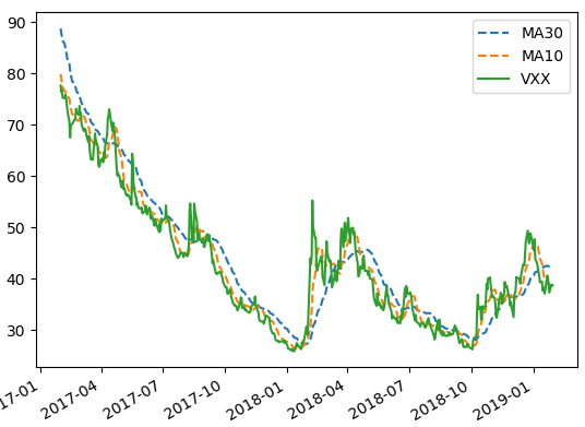
If 10-day Moving Average (MA10) < 30-day Moving Average (MA30) Sell Short

If 10-day Moving Average (MA10) >= 30-day Moving Average (MA30) Cover Short

The system is implemented in Python. Graph above shows the MAs and VXX for the last 2 years

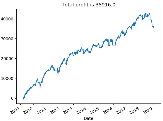
The position size is $10000; leverage is not utilized, and profit is not compounded. Graph below shows the equity curve for the trading strategy from January 2009 to January 2019.

References

[1]  E. Sinclair, Volatility Trading, John Wiley & Sons, 2008

 

Article Source Here: Quantitative Trading