Monday, November 30, 2020

Modern Portfolio Theory-Portfolio Management in Python

Harry M. Markowitz is the founder of Modern Portfolio Theory (MPT) which originated from his 1952 essay on portfolio selection. He was later awarded a Nobel Prize in Economics. His work founded the concept of an efficient frontier, and it allows for the determination of portfolio mixes that provide an optimal return for the least amount of risk.

Modern portfolio theory (MPT), or mean-variance analysis, is a mathematical framework for assembling a portfolio of assets such that the expected return is maximized for a given level of risk. It is a formalization and extension of diversification in investing, the idea that owning different kinds of financial assets is less risky than owning only one type. Its key insight is that an asset's risk and return should not be assessed by itself, but by how it contributes to a portfolio's overall risk and return. It uses the variance of asset prices as a proxy for risk. Read more

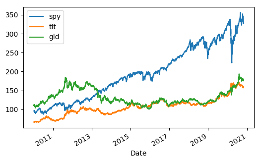
In this post, we are going to provide a concrete example of implementing MPT in Python. Our portfolio consists of 3 Exchange Traded Funds (ETF): SPY, TLT, and GLD which track the S&P500, long-term Treasury bond, and gold respectively.  We downloaded 10 years of data from Yahoo Finance. The picture below shows the price time series of the 3 ETFs.
Modern Portfolio Theory in Python

We utilized Python to calculate each EFT expected return and volatility. We then assigned a random weight to each ETF and determined the portfolio’s expected return and volatility. Recall that,

MPT assumes that investors are risk averse, meaning that given two portfolios that offer the same expected return, investors will prefer the less risky one. Thus, an investor will take on increased risk only if compensated by higher expected returns. Conversely, an investor who wants higher expected returns must accept more risk. The exact trade-off will not be the same for all investors. Different investors will evaluate the trade-off differently based on individual risk aversion characteristics. The implication is that a rational investor will not invest in a portfolio if a second portfolio exists with a more favorable risk-expected return profile – i.e., if for that level of risk an alternative portfolio exists that has better expected returns.

Under the model:

  • Portfolio return is the proportion-weighted combination of the constituent assets' returns.
  • Portfolio volatility is a function of the correlations ρij of the component assets, for all asset pairs (i, j).

We repeated the above process many times and obtained the following return/risk profile for possible portfolios.
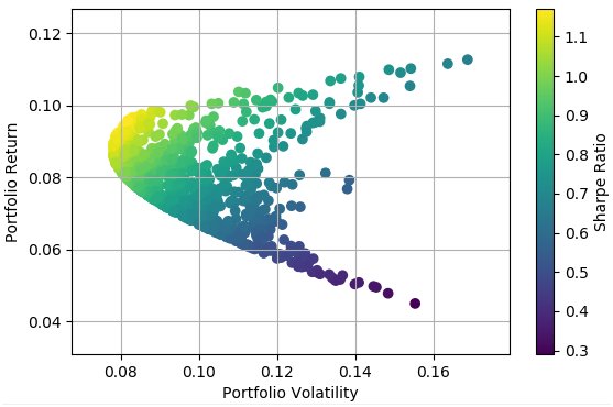
Portfolio Management in Python

In the next installment, we will search for an optimal portfolio that provides the highest return for the least amount of risk.

Click on the link below to download the Python program.

Article Source Here: Modern Portfolio Theory-Portfolio Management in Python


Saturday, November 28, 2020

Statistical Analysis of an ETF Pair-Quantitative Trading In Python

Pair trading, or statistical arbitrage, is one of the oldest forms of quantitative trading. In this post, we are going to present some relevant statistical tests for analyzing the Australia/Canada pair. We chose this pair because these countries’ economies are tied strongly to the commodity sector, therefore they share similar characteristics and could be a good candidate for pair trading.

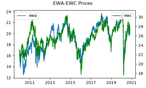
We first downloaded the data from Yahoo Finance. We downloaded 10 years of data of EWA and EWC, which are the Exchange Traded Funds (ETF) associated with Australia and Canada, respectively.  We then utilized Python to plot the data and perform statistical tests.

The chart below shows the price time series. Visually, these 2 country ETFs move in a similar fashion, more or less.

Quantitative Trading In Python

We next calculated the correlation of returns and obtained 0.7908. The high correlation makes the pair a good candidate for statistical arbitrage.

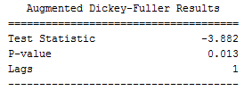
We then determined the price spread and performed the Augmented Dicker Fuller test for cointegration.

In statistics and econometrics, an augmented Dickey–Fuller test (ADF) tests the null hypothesis that a unit root is present in a time series sample. The alternative hypothesis is different depending on which version of the test is used, but is usually stationarity or trend-stationarity. It is an augmented version of the Dickey–Fuller test for a larger and more complicated set of time series models.

The augmented Dickey–Fuller (ADF) statistic, used in the test, is a negative number. The more negative it is, the stronger the rejection of the hypothesis that there is a unit root at some level of confidence. Read more

The picture below shows the test results. The p-value is less than 0.05; therefore the pair is cointegrated at the 95% confidence level.

cointegration test in python

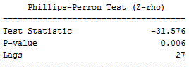
Finally, we performed the Phillips-Perron test for cointegration on the spread.

In statistics, the Phillips–Perron test (named after Peter C. B. Phillips and Pierre Perron) is a unit root test. That is, it is used in time series analysis to test the null hypothesis that a time series is integrated of order 1... Like the augmented Dickey–Fuller test, the Phillips–Perron test addresses the issue that the process generating data for yt might have a higher order of autocorrelation than is admitted in the test equation—making yt-1 endogenous and thus invalidating the Dickey–Fuller t-test. Read more

The picture below shows the test results. The p-value is less than 0.05; therefore the pair is cointegrated at the 95% confidence level.

cointegration analysis in python

In the next installment, we will implement a trading strategy using this cointegrated pair.


Click on the link below to download the Python program.

Article Source Here: Statistical Analysis of an ETF Pair-Quantitative Trading In Python


Tuesday, November 24, 2020

Capital Asset Pricing Model

The Capital Asset Pricing Model (CAPM) is a model that investors use to determine the rate of return of an investment. The model describes the relationship between the expected return of an investment and its risks. Furthermore, CAPM is one of the most commonly used models in finance for pricing risky stocks. Both investors and businesses use the model to calculate their rate of return.

For investors, CAPM can help with the calculation of the required rate of return. More importantly, it can help them develop a diversified portfolio of investments. For companies and businesses, CAPM helps with the calculation of the cost of equity. They can use the cost of equity in different processes such as investment appraisal or in the calculation of Weighted Average Cost of Capital (WACC).

Capital Asset Pricing Formula

To calculate the rate of return using CAPM investors and businesses use the following formula.

E(r)i = Rf + βi (E(r)m - Rf)

In the above formula, ‘E(r)i’ represents the expected rate of return of an investment or stock. ‘Rf' signifies the risk-free rate of return prevalent in the market. 'βi’ represents the beta of the investment. Finally, ‘E(r)m' denotes the average rate of return in the market. Together, (E(r)m - Rf) represents the market risk premium.

Risk-free rate of return

The risk-free rate of return is the rate of return of a risk-free investment. Usually, it represents a theoretical rate of return and is close to the rate of return of short-term government treasury bills. For most calculations, investors can use the rate of return on those treasury bills instead of calculating the risk-free rate of return.

Beta

The most important part of the CAPM model is the Beta factor or coefficient of an investment. Beta represents the systematic risk of an investment. Systematic risk is the risk that applies to the market as a whole and not to a specific company or stock. Usually, companies with a beta of above 1 are riskier than the market. A beta of lower than 1 represents a lower risk than the market.

Market risk premium

The market risk premium of an investment represents the premium above the risk-free rate of return in the market. It is calculated by deducting the risk-free rate of return from the average market rate of return. In simpler words, the market risk premium is the difference between the average market rate of return and the risk-free rate of return.

Advantages of using CAPM

There are many advantages to using CAPM. First of all, it is easy to use. All the figures required in its calculations are available in the market. Similarly, the model is also useful because it takes into account the systematic risk of investments or stocks. Through these, CAPM allows investors to diversify their portfolio and eliminate unsystematic risk.

Disadvantages of using CAPM

There are also some disadvantages to using CAPM. These disadvantages come from the assumptions made by the model or its dependencies. First of all, CAPM assumes there is a risk-free rate of return, which is not possible. Similarly, for some investments calculating beta may not be possible. Therefore, it may limit the model.

Conclusion

The Capital Asset Pricing model can help investors determine the required rate of return of an investment. It is useful for both investors and businesses. To calculate the rate of return, investors must use the CAPM formula given above.

Article Source Here: Capital Asset Pricing Model


Sunday, November 22, 2020

Formula for Dividend Yield

The dividend yield is a financial ratio that represents the annual dividends paid to shareholders against a stock in relation to its current market price. In simpler words, the dividend yield measures a company's dividends as a percentage of its stocks' current market price.

The dividend yield is a useful formula for investors and shareholders to determine how much dividends they can expect in the future. As the ratio is different for various industries and companies, it plays a critical part in the decision-making process of investors and shareholders. Usually, stable or mature companies will have better dividend yields as compared to startups.

Dividend yield formula

The formula for dividend yield is straightforward. Investors can use the formula below to calculate it.

Dividend yield = Annual dividends per share / Market value per share

In the above formula, the annual dividends per share represent the total dividends paid out by the company divided by its number of outstanding shares. Similarly, the market value per share represents the share price of the company at the time of evaluation.

Example

A company, Banana Co. paid total dividends of $10,000 in its last accounting period. Its total outstanding number of shares at the time was 5,000 shares. The current market price of Banana Co.'s share in the stock market is $100. Therefore, its dividend yield will be.

Dividend yield = Annual dividends per share / Market value per share

Dividend yield = ($10,000 / 5,000) / $100

Dividend yield = 0.02 or 2%

Meaning of dividend yield

The dividend yield, as stated above, shows the percentage of the market value of a share paid in dividends. Therefore, the higher the dividend yield of a stock is, the better it is. For example, a company that has a dividend yield of 10% is preferable to investors as compared to companies that pay below that. However, it does not only stop there.

Some companies may have fluctuations in their dividend yields over time. Usually, if a company's dividend yields increase each year, it means the company has been growing. However, it may also imply that the company's share prices are dropping in the market. Similarly, declining dividend yields also do not mean decreasing dividends. Therefore, investors need to be aware of the causes behind the fluctuations.

Importance of dividend yield

The dividend yield is a vital ratio for dividend investors. Investors that rely on steady dividends may base their investing decisions on the dividends paid by the company. Therefore, the dividend yield is critical in their decision-making process. For growth investors, however, dividend yield may not be as important.

Limitations of dividend yield

The dividend yield, as a financial metric, may have some limitations. As mentioned above, while higher dividend yields are preferable, they are not necessarily an indicator of higher dividends. Similarly, the dividend yield may not be an indicator of a better performance of the company. Usually, paying high dividends means the company is not investing in future activities, which can worsen the future prospects of investments.

Conclusion

The dividend yield is a metric used to calculate the percentage of dividends of a company over its current market price. Usually, investors prefer a higher dividend yield stock. However, there may be some other issues they must consider as well.

Originally Published Here: Formula for Dividend Yield


Saturday, November 21, 2020

Arbitrage Pricing Theory

The Arbitrage Pricing Theory (APT) is a model that describes the relationship between the expected returns from an asset and its risks. Often used as an alternative to the Capital Asset Pricing Model (CAPM), APT is a multi-factor model for investments that explains the risk-return relationship using various independent factors rather than relying on a single index, as with CAPM.

While this model got developed in 1976, much after CAPM, however, many investors still use the latter for their calculations. As compared to CAPM, the APT uses less restrictive assumptions, which gives it an advantage over CAPM. While the APT uses a multi-index approach to calculations, it does not specify what the index should be, which is its downside compared to CAPM, which does.

Arbitrage Pricing Theory Formula

The formula to calculate the expected return using APT depends on how many factors or indexes investors take into account. Therefore, it can be represented as follows.

E(r)i = Rf + β1RP1 + β2RP2 + β3RP3 + … + βnRPn

In the above formula, “E(r)i” represents the return calculated by the model. “Rf” denotes the risk-free rate of return. “βx” symbolizes the beta for a specific index or factor considered. “RPx" represents the risk premium of the considered index. Finally, "n" denotes the number of indexes considered by the investor.

There are two types of factors that the model considers. These include macroeconomic factors, such as inflation, GDP, etc., and factors specific to the market or stock. The market-specific risks consist of systematic risks associated with the stock in question.

Assumptions of Arbitrage Pricing Theory

There are three assumptions that APT makes when calculating return on an asset. First of all, it assumes that returns depend only on systematic factors. Similarly, the model assumes that no-arbitrage exists. In case there are any arbitrage opportunities, the market will exploit them. Lastly, APT implies that investors can build a portfolio of diversified assets, thus, eliminating any specific risks in the process.

Advantages of using Arbitrage Pricing Theory

There are many advantages of using APT to determine the expected return. First of all, APT allows investors to use several factors rather than be limited to one. The model also does not specify the factors, allowing investors the choice to weigh in factors of their choice.

Similarly, it has fewer restrictions as compared to some other models. Likewise, the model also provides much better compensation for unforeseen circumstances. Lastly, the model provides investors with an opportunity to identify and exploit arbitrage opportunities.

Disadvantages of using Arbitrage Pricing Theory

Despite its advantages, APT may also come with some disadvantages. First of all, some investors may consider APT more complicated as compared to other models. Similarly, APT requires risk sources to be accurate to produce accurate results. Despite all the calculations, however, the model still does not guarantee results.

Conclusion

Arbitrage Pricing Theory (APT) is a model used in the calculation of the return of investments. It is considered an alternative to the well-known Capital Asset Pricing Model (CAPM). However, unlike CAPM, APT weighs multiple factors or indexes when calculating an expected return.

Originally Published Here: Arbitrage Pricing Theory


Friday, November 20, 2020

P/E Ratio of Stocks

The price-to-earnings (P/E) ratio represents the relationship between the market value of the stock of a company and its earnings per share (EPS). It is one of the most commonly used and well-known ratios used by investors in valuing the stocks of a company. Other names for the P/E ratio are the price multiple or earnings multiple.

P/E ratio formula

The formula to calculate the P/E ratio is straightforward and is as follows.

P/E ratio = Market price of stock / Earnings Per Share

The market price of the stock shows its current price in the stock market. Usually, this market price of a stock is readily available from the stock market. The Earnings Per Share (EPS) represent the total earnings of a company divided by its total shares in the last accounting period. The EPS of a company is available in its financial statements, usually in the Income Statement.

Example

A company named Red Co. has a current market stock price of $100. In the previous accounting period, Red Co. had total earnings of $100 million while its outstanding shares in the market were 20 million shares. Therefore, the company's EPS was $5 per share ($100 million/20 million shares). The P/E ratio of Red Co. is as follows.

P/E ratio = Market price of stock / Earnings Per Share

P/E ratio = $100 / $5

P/E ratio = 20 (times)

Meaning of P/E ratio

When investors use the P/E ratio to evaluate their investments, they must understand what it means. A high P/E ratio signifies that the market trusts the company will grow in the future. Therefore, the market participants are willing to pay higher for the company's stocks despite the low EPS. However, investing in high P/E ratio stocks also presents higher risks as the growth potential may not capitalize.

Similarly, a low P/E ratio means that the stock of a company is undervalued. These usually represent value stocks in which investors may want to invest. Usually, the reason behind a low P/E is mispricing and can result in outstanding gains once it recovers to its correct value in the market. It may also indicate a company is doing well compared to its past trends.

It is crucial to use the P/E ratio as a comparison tool to make better use of it. P/E ratio cannot give a meaningful result on its own. Therefore, investors must obtain the P/E ratio for different stocks and compare them. Based on their risk preferences, investors can then make decisions in which stock they want to invest. Similarly, it is better to use the P/E ratio to compare between similar stocks, for example, companies within the same industry, for best results.

Limitations of P/E ratio

The P/E ratio has some limitations. First of all, the ratio requires investors to determine the price or EPS of a stock, which may not be possible for every company. For example, for private companies, the information may not be readily available. Similarly, some companies may have volatile market stock prices, which can affect the calculations. The ratio also fails to consider the earning growth of stocks.

Conclusion

P/E, or price-to-earnings ratio, represents the price of a stock in relation to the EPS of the company to which it relates. It is one of the most favourite tools used by investors when making decisions about their investments.

Originally Published Here: P/E Ratio of Stocks


Thursday, November 12, 2020

What It Takes to Win at Quantitative Investing

A recent podcast on Bloomberg offers some interesting perspectives on quantitative investing.

Interest in quantitative investing strategies continues to grow; however, as the space gets more competitive, making money and winning gets harder and harder. Computation costs alone can be prohibitive. On the latest episode, we speak with Columbia Business School professor Ciamac Moallemi about how the world's best quant funds thrive.

quantitative trading

The key takeaways are,

  • Quantitative investing has two key characteristics. The first characteristic is that the investment process is entirely systematic. The second characteristic is that quantitative strategies are active investment strategies.
  • The market is inefficiently efficient, or efficiently inefficient, meaning that there exist inefficiencies, but it's a competitive game, and there are lots of smart people with a lot of resources out there who are going after these inefficiencies, and when they identify them and trade on them, the inefficiencies will disappear.
  • The key to winning in quantitative investing is not about identifying some flaws in the market or some inefficiencies or some opportunities to make money. It's about having a team and a process to keep finding those over and over again.
  • Historically, much of quantitative investing has been built on what was called “technical models”, where basically you're using historical price and trade data to forecast future price movements. What we have seen emerge over the past 10 years is a shift towards alternative data.
  • Quantitative investors operate quite differently than research groups in big tech places. Research conducted in laboratories of big tech companies like Google, Microsoft, or Bell is not that different than in an academic institution. The main output is publication in research journals and conference papers. In the quant world, the research process is, however, much more applied, and there is no incentive for publishing research results.
  • What value does quantitative investing actually create for society? Quantitative investing is about arbitraging the small inefficiencies, so maybe it will make prices slightly more efficient. But is that worth the enormous infrastructure investment being spent on it?

Originally Published Here: What It Takes to Win at Quantitative Investing

Monday, November 2, 2020

Enterprise Value to EBITDA Multiple

Introduction

The Enterprise Value to EBITDA ratio, also known as the EBITDA multiple, is a ratio used to measure the value of a company. Usually, the reason for calculating the EV/EBITDA ratio is to use it as a comparison tool between different companies. It can also be helpful in other techniques, such as Comparable Company Analysis. The multiple has two components, Enterprise Value and EBITDA.

Enterprise Value (EV) is a measure of the total value of a company. EV is the sum of the current market capitalization of a company, its debt, minority interest, and preferred shares, less its cash and cash equivalents. On the other hand, EBITDA represents the earnings of a company before considering its interest, taxes, depreciation, and amortization.

Uses of Enterprise Value to EBITDA Multiple

As mentioned above, the EV/EBITDA multiple can help in comparing the value of different companies. This ratio can help investors determine how many times the EBITDA of a company they have to pay if they want to acquire the company. It can also help in the calculation of the terminal value in the Discounted Cash Flow (DCF) model. Finally, it can also help in calculating a target price for a company in an equity research report.

Advantages of Enterprise Value to EBITDA Multiple

There are many advantages of using EV/EBITDA multiple. First of all, it is easy to calculate and the information required to calculate it is readily available. Secondly, as mentioned above, it can help provide a comparison between the values of different companies. Most experts also prefer the EV/EBITDA ratio as compared to other metrics such as the Price to Earnings ratio. Finally, the multiple works great for valuing a well-established business with low capital expenditures.

Disadvantages of Enterprise Value to EBITDA Multiple

The EV/EBITDA multiple may also have some disadvantages. First of all, it does not take into account the assets or capital expenditures of a company. It is also not a good proxy for cash flow due to its use of the EBITDA. It is also hard to adjust for companies with different growth rates. The ratio is also susceptible to manipulation due to its use of EBITDA.

Example

A company has an Enterprise Value of $300 million and an EBITDA of $30 million. It can calculate its EV/EBITDA multiple in the following way.

EV/EBITDA multiple = Enterprise Value / EBITDA

EV/EBITDA multiple = $300 million / $30 million

EV/EBITDA multiple = 10 times

In this example, the EV and EBITDA are already available. However, practically, these figures are not available beforehand and need to be calculated. For instance, if investors want to calculate the multiple, they must obtain the current market capitalization, debt, minority interest, and value of preferred shares of a company. After that, they need to deduct cash and cash equivalents from the sum of those amounts. Similarly, they must add the interest, taxes, depreciation, and amortization of the company to its earnings to obtain its EBITDA.

Conclusion

The EV/EBITDA multiple is a ratio calculated by dividing the Enterprise Value (EV) of a company by its EBITDA. It has different uses, including being used to calculate the value of a company and as a comparison tool. There are many advantages of using the multiple. However, it may have its disadvantages as well.

Originally Published Here: Enterprise Value to EBITDA Multiple

Sunday, November 1, 2020

Comparative Company Analysis

Introduction

Comparative Company Analysis (CCA) is a process used to compare two similar companies, operating in the same industry. It is a valuation methodology that allows users to evaluate the ratios of similar public companies and use those ratios to derive the value of another company. CCA assists users in determining the relative value of a company. It is different from other methods that allow users to determine the intrinsic value of a company, such as Discounted Cash Flow analysis.

How to perform Comparative Company Analysis?

Performing CCA is simple and straightforward. First of all, users need to analyze different companies and obtain those that are suitable for comparison. This process needs them to perform some research and also requires some judgment on their part. When trying to find companies for comparison, users should consider companies that are in the same industry and geographical location. Usually, CCA works best for companies that are competitors.

Once the user selects different companies to use in CCA, the next step is to obtain their financial statements and other financial information. For public listed companies, these are available in their relevant stock markets or their websites. For private listed companies, the financial statements may be difficult to obtain. Usually, private listed companies also have their financial statements on their websites. However, for some others, they may not be available at all.

Once the user obtains the required financial information of the selected companies, the process of comparative analysis begins. Users can use different metrics to compare those companies. These metrics include share price, market capitalization, Enterprise Value (EV), revenues, net profits, EBITDA, EPS, etc. Similarly, users can also calculate different ratios for companies. These ratios may include EV/EBITDA, EV/Revenue, Price to Earnings, Price to Book value, etc. There are online templates available that users can also use as a base for CCA.

Finally, users can interpret the information from the CCA to make decisions regarding the company in question. Usually, the interpretation and decision depend on the needs of the users. There are no specific rules regarding how they should interpret the information. CCA can only help users analyze quantitative information. Therefore, users must understand that the results obtained through CCA will not consider qualitative factors.

Advantages of Comparable Company Analysis

Comparable Company Analysis can help users determine a benchmark value-based on the firm valuation. It provides them with a tool to compare and assess the financial performance of different companies better. The information obtained through CCA relates to real market data. Therefore, it is better than other tools that depend on estimations and forecasts. Furthermore, CCA is easy to calculate and explain, making it a superb tool for users of all levels.

Disadvantages of Comparable Company Analysis

The main disadvantage of CCA is that it requires many different companies for the best results. If there are a few comparable companies, the tool may not provide accurate results. Similarly, which companies qualify for comparison depends on the users’ judgment. Furthermore, there are no companies that one may consider truly comparable.

Conclusion

Comparable Company Analysis is a tool that allows users to compare similar companies in the same industry. For CCA, users need to select similar companies first and obtain financial information about them, including their financial statements. Then they can use different metrics and ratios to compare these companies. The interpretation of these comparisons depends on the needs of the users. CCA may have some advantages and disadvantages, given above.

Originally Published Here: Comparative Company Analysis