Saturday, October 31, 2020

Forecasting Implied Volatility with ARIMA Model-Volatility Analysis in Python

In a previous post, we presented theory and a practical example of calculating implied volatility for a given stock option. In this post, we are going to implement a model for forecasting the implied volatility. Specifically, we are going to use the Autoregressive Integrated Moving Average (ARIMA) model to forecast the volatility index, VIX.

In statistics and econometrics, and in particular in time series analysis, an autoregressive integrated moving average (ARIMA) model is a generalization of an autoregressive moving average (ARMA) model. Both of these models are fitted to time series data either to better understand the data or to predict future points in the series (forecasting). ARIMA models are applied in some cases where data show evidence of non-stationarity, where an initial differencing step (corresponding to the "integrated" part of the model) can be applied one or more times to eliminate the non-stationarity.

The AR part of ARIMA indicates that the evolving variable of interest is regressed on its own lagged (i.e., prior) values. The MA part indicates that the regression error is actually a linear combination of error terms whose values occurred contemporaneously and at various times in the past. The I (for "integrated") indicates that the data values have been replaced with the difference between their values and the previous values (and this differencing process may have been performed more than once). The purpose of each of these features is to make the model fit the data as well as possible. Read more

It is shown in Reference [1] that the implied volatility index can be modeled and forecasted using the ARIMA model. To apply the ARIMA model to the VIX index, we first downloaded 5 years of historical data of the VIX from Yahoo Finance. Next, we used the first 4 years of data as the training set and fit the data to the ARIMA model. The Python SARIMA program returned the following model parameters,

Implied volatility analysis in python

After obtaining the parameters, we applied the model to the remaining 1 year of data and calculated the forecasted VIX on a rolling window of 1 month. The picture below shows the rolling forecasted VIX along with the VIX index,
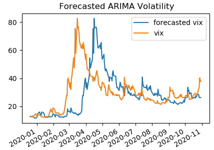
Volatility trading in python with ARIMA

Click on the link below to download the Python program.

References

[1]  K. Ahoniemi,  Modeling and forecasting implied volatility, Helsinki School of Economics, 2009.

Post Source Here: Forecasting Implied Volatility with ARIMA Model-Volatility Analysis in Python

Friday, October 30, 2020

FASB Proposes Scope Clarification for Reference Rate Relief

On July 27, 2017 the Financial Conduct Authority, the U.K.'s top regulator, tasked with overseeing Libor, announced the benchmark will be phased out by 2021. Alternative risk-free rates are being set up for the different currencies. For the US Dollar, the US Fed's Alternative Reference Rates Committee (ARRC) has recommended using the Secured Overnight Financing Rate (SOFR), which has been published since April 2019.[86] For the British Pound, it is the Sterling Over Night Index Average (SONIA), and for the Euro, the Euro Short-Term Rate (€STR).Regulators are now expecting financial institutions to actively prepare for the cessation of LIBOR and the adoption of alternative risk-free rates. The FCA and Prudential Regulation Authority (PRA) were the first regulators globally to ask firms for their preparation and actions to manage the LIBOR transition, in a September 2018 letter. Other regulators, including the European Central Bank's supervisory board, followed. ISDA has run several consultations to improve the fallback process. Read more

FASB issued a proposal Thursday that is intended to clarify the scope of the board’s guidance on reference rate reform.

In March, FASB issued Accounting Standards Update No. 2020-04, Reference Rate Reform (Topic 848): Facilitation of the Effects of Reference Rate Reform on Financial Reporting. The standard was issued to address accounting challenges resulting from the sunsetting of the London Interbank Offered Rate (LIBOR) as well other benchmark interest rates banks use to make short-term loans to one another.

FASB ASC Topic 848 provides temporary, optional expedients and exceptions for using GAAP to contract modifications and hedging relationships that reference LIBOR or another reference rate that is expected to be discontinued. Read more

Post Source Here: FASB Proposes Scope Clarification for Reference Rate Relief

Thursday, October 29, 2020

Discounted Cash Flow Model

Introduction

The Discounted Cash Flow (DCF) model is a method that investors use to estimate the value of an investment based on future cash flows. The DCF model uses the forecasted cash flows of investment to determine its value today. However, this tool isn't only for investors. Business owners and company shareholders can also use the DCF model to make decisions related to their existing companies in businesses.

The DCF model depends on a concept known as the time value of money. That's what the 'discounted' part of its name means. According to the time value of money concept, cash flows generated today are worth more than those generated in the future. Therefore, it requires users to discount cash flows using a rate of return, or cost of capital, for better decision-making.

Uses of Discounted Cash Flow Model

As mentioned above, there are many uses of the discounted cash flow model. Firstly, investors can use it to estimate the present value of an investment, which allows them to make better decisions. Companies may also use it to evaluate different projects and compare them with each other. The DCF model helps companies estimate the actual value of an investment, taking into consideration the time value of value, rather than its perceived value.

Some examples of how different entities can use the DCF model include determining the value of a company or a project. It may also include determining the value of the shares, bonds, and other instruments of a company. In short, the DCF model can be used to estimate the intrinsic value of any project or investment that generates cash flows.

Disadvantages of Discounted Cash Flow Model

The DCF model can also have some disadvantages. The model requires users to make different estimates. These estimates include forecasting cash flows of an investment or project, or the rate of return to use. Estimating these amounts is not as straightforward as they depend on certain internal and external factors. Therefore, a misestimation in these values can change the outcome of the decisions made by an entity.

Discount Cash Flow Model formula

The formula to calculate the cash flows of a particular instrument, investment, or project using the DCF model is straightforward. It involves discounting all the cash flows using an appropriate rate of return or cost of capital. Usually, calculating the present value of cash flows using the DCF model requires a proper structure, using a spreadsheet program. However, the formula can be presented as below.

DCF = [CF­­1 x (1+r)-1] + [CF2 x (1+r)-2] + … + [CFn x (1+r)-n]

In the above formula ‘CF’ represents the cash flow for each year. ‘r’ represents the required rate of return or cost of capital of a particular project or investment. Lastly, ‘n’ represents the total number of years of the project.

Example

A company wants to assess a 5-year particular project. The cost of capital of the company is 10%. The estimated cash flows from the project are as below.

Year

Cash flow

1

       150,000

2

       120,000

3

       100,000

4

         60,000

5

         50,000

       480,000

Using the DCF model, the company can calculate the present value of all cash flows using the 10% cost of capital. The calculation is as below.

Year Cash flow Discount factor (10%) Present value
1        150,000 0.909   136,350
2        120,000 0.826     99,120
3        100,000 0.751     75,100
4          60,000 0.683     40,980
5          50,000 0.621     31,050
       480,000   382,600

Conclusion

The Discounted Cash Flow (DCF) model is a tool used to calculate the present values of the cash flows from a particular project or investment. Investors, shareholders, and companies use the model to determine the value of a particular investment or project. However, the model works with assumptions, which may affect the calculations.

Originally Published Here: Discounted Cash Flow Model

Wednesday, October 28, 2020

EBITDA, What It Is and How to Calculate It

Introduction

EBITDA, short for Earnings Before Interest, Taxes, Depreciation, and Amortization, is an indicator of the financial performance of a company. It is an alternative to the traditional measures of a company's performance, such as operating profits. Similarly, it is also considered an alternative for the operational cash flows of a company. EBITDA is one of the many variations of the EBIT metric.

Importance of EBITDA

EBITDA is a crucial metric for investors and businesses. The metric gives investors a quick estimate of the value of a specific company. Besides, companies that suffer in converting revenues into profits can still have a positive EBITDA. That is because EBITDA considers the earnings of a company before considering items that are outside its control. Therefore, investors can use EBITDA to determine whether the losses made by a company related to operating deficiencies or other factors.

Similarly, EBITDA is also vital because it allows investors to compare between different companies in a better way. However, they can only use it to compare similar companies operating in the same industry. Furthermore, it can also allow companies to compare their performance against competitors and other similar companies to identify any problems within their processes.

Problems with EBITDA

Using EBITDA can also have some problems. Firstly, EBITDA is not an officially recognized metric by any accounting standard. Similarly, some experts believe that taking out depreciation from EBITDA disregards the lost value of assets over time. Therefore, it can produce inaccurate results, especially for companies that acquire many assets over time through the use of debt instruments.

How to calculate EBITDA?

The calculation of EBITDA is straightforward. The formula to calculate EBITDA is below.

EBITDA = Earnings + Interest + Taxes + Depreciation + Amortization

The figures required in calculating EBITDA are available in the financial statements of a company. The earnings, interest, and tax amounts are available in the Statement of Profit or Loss of companies. The figures for depreciation and amortization are obtainable from the Notes to the Financial Statements.

There’s also an alternative formula to calculate EBITDA, given below.

EBITDA = Operating profit + Depreciation + Amortization

The operating profit of a company is its profit before interest and taxes, also referred to as EBIT, available in its Statement of Profit or Loss.

Example

A company has earnings of $100 million. It charged interest expense of $7 million, taxes amounting to $3 million, depreciation of $10 million, and amortization of $5 million in its financial statements. To calculate its EBITDA, the company can use the following formula.

EBITDA = Earnings + Interest + Taxes + Depreciation + Amortization

EBITDA = $100 million + $7 million + $3 million + $10 million + $5 million

EBITDA = $125 million

Conclusion

EBITDA is a metric widely used as an indicator of the financial performance of a company. EBITDA stands for Earnings Before Interest, Taxes, Depreciation, and Amortization. There are many different uses of EBITDA, although it may come with some problems. There are two formulas used in the calculation of the EBITDA of a company.

Originally Published Here: EBITDA, What It Is and How to Calculate It

Tuesday, October 27, 2020

Preferred Shares vs Common Shares

Introduction

When it comes to the shares of companies, there are two commonly available types in the market. These include common shares and preferred shares. While they both give shareholders certain rights, there are some differences between them. Therefore, it is crucial to understand the differences between them.

What are Common Shares?

Common shares sometimes referred to as ordinary shares, are the most commonly traded shares of companies. Usually, when people talk about the shares of a company, they refer to common shares. Most companies around the world only issue ordinary shares. Common shares give shareholders partial ownership of a company. It also comes with certain voting rights, which allows common shareholders to choose the board of directors of a company.

Apart from voting rights, common shareholders also get the right to receive dividends. Dividends are the distribution of the profits of a company to its shareholders. Some companies may not distribute dividends at all. However, most others do pay their shareholders regular dividends, usually at the end of each accounting period.

However, dividends aren't the only type of return that common shareholders get. Common shareholders can also benefit from an increase in the price of the shares of a company, which can result in capital gains for them. Capital gains happen with the market price of the shares of a company exceed the price paid by the shareholders originally.

Finally, common shares also give rights to the assets of a company in case of liquidation. However, there are some conditions attached to the assets they can receive. For example, in the case of liquidation, a company must pay all its debts first. After the repayment of these debts, if the company has any assets remaining, it is distributed to its shareholders.

What are Preferred Shares?

Preferred shares are different from common shares due to many reasons. Companies issue preferred shares less frequently as compared to common shares. Furthermore, preferred shares give the shareholder a preference over ordinary shareholders. However, they do not come with voting rights, unlike common shares. Therefore, preference shareholders cannot take part in selecting the board of directors of a company.

When it comes to dividends, preferred shares come with an advantage. Usually, preference shareholders receive a higher dividend as compared to common shareholders. Similarly, the dividend that companies pay to their preferred shareholders is predetermined, unlike common shares. When paying dividends, companies must pay preferred shareholders first and any remaining amount to common shareholders.

While preferred shares can still generate a capital gain for shareholders, they do not appreciate in value as much as common shares. Therefore, preferred shareholders don’t usually rely on capital gains but mostly buy preferred shares for dividends. The market price and capital gain on preferred shares also depend on how close they are to maturity.

Finally, in case a company liquidates, preferred shareholders get an advantage over ordinary shareholders. As mentioned above, companies must pay their debts first when liquidated. However, after paying these debts, they must first compensate their preferred shareholders. Any remaining amount after they pay off their debts and preferred shareholders are attributable to common shareholders.

Valuing Preferred Shares

The valuation of preferred shares is different from the valuation of common shares. Preferred shares can be valued using the same valuation method as convertible and/or callable bonds.

Conclusion

Common or ordinary shares are shares that give partial ownership of the company to shareholders. On the other hand, preferred shares are also similar but come with a preference over common shares. Both of them are different due to many reasons. These include differences in voting rights, dividends, capital gains, and preference at liquidation.

Post Source Here: Preferred Shares vs Common Shares

Monday, October 26, 2020

Forecasting Volatility with GARCH Model-Volatility Analysis in Python

In a previous post, we presented an example of volatility analysis using Close-to-Close historical volatility. In this post, we are going to use the Generalized Autoregressive Conditional Heteroskedasticity (GARCH) model to forecast volatility.

In econometrics, the autoregressive conditional heteroscedasticity (ARCH) model is a statistical model for time series data that describes the variance of the current error term or innovation as a function of the actual sizes of the previous time periods' error terms; often the variance is related to the squares of the previous innovations. The ARCH model is appropriate when the error variance in a time series follows an autoregressive (AR) model; if an autoregressive moving average (ARMA) model is assumed for the error variance, the model is a generalized autoregressive conditional heteroskedasticity (GARCH) model.

ARCH models are commonly employed in modeling financial time series that exhibit time-varying volatility and volatility clustering, i.e. periods of swings interspersed with periods of relative calm. ARCH-type models are sometimes considered to be in the family of stochastic volatility models, although this is strictly incorrect since at time t the volatility is completely pre-determined (deterministic) given previous values.  Read more

As an example, we are going to apply the GARCH model to the SP500. We first downloaded 5 years of historical data of SPY from Yahoo Finance. Next, we used the first 4 years of data as the training set and fit the data to the GARCH (1, 1) model. The Python ARCH program returned the following model parameters,

GARCH volatility model in python

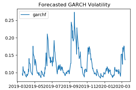
After obtaining the parameters, we applied the model to the remaining 1 year of data and calculated the forecasted volatility on a rolling window of 1 month. The picture below shows the rolling forecasted volatility,

GARCH volatility trading in python

Click on the link below to download the Python program.

Post Source Here: Forecasting Volatility with GARCH Model-Volatility Analysis in Python

Wednesday, October 21, 2020

Accounting for Stock Warrants

A stock warrant is a contract between a company and investors, which gives them the right to purchase newly issued shares of a stock at a set price for a set period of time. The company directly issues the new stock instead of using issued stock. However, investors that get a stock warrant do not have a legal right to the ownership of stock, but only a right to purchase it in the future. Similarly, for the company, a stock warrant does not lock in investors to buy the stock. They still have a choice of not exercising the right.

Since the warrant sets the price of the newly issued stock, it can be beneficial to the investors. Especially when the price of the company's stock rises in the stock market, investors can profit from the lower price of stocks offered to them through warrants. Similarly, the market price of the stock of a company will not affect the price of the warrant, as the company issues the new stocks, and the price is preset.

There are many different types of stock warrants that companies may put into use. The two main types of stock warrants are put and call warrants. A put warrant limits the amount of equity that the investor can sell back to the company at a given price. A call warrant, on the other hand, guarantees the investor’s right to purchase a predetermined number of shares at a predetermined price. There are also other types of warrants such as covered, naked, traditional, and wedded warrants. These are classified based on the degree of risk and value of the warrant.

Accounting for Stock Warrants

When it comes to accounting for stock warrants, the company issuing them must ensure two things. First, the company must recognize the fair value of the equity instrument issued or the fair value of the consideration received, based on whichever is reliably measurable. Second, the company must recognize the asset or expense related to the goods or services at the same time.

If the option to exercise the stock warrant expires, the company cannot reverse the related expense or asset recognized. Furthermore, if a company receives warrants in exchange for products or services, it can recognize revenues normally, as they would under the accounting standard related to revenue.

Once the company determines the fair value of the stock warrant, the company can use the following accounting treatment to account for the transaction.

Dr Expense/Asset

Cr Stock warrants

When the investor exercises the option to avail the stock warrants, the company can use the following accounting treatment to convert the stock warrant balance into equity.

Dr Stock warrants

Cr Share capital

Cr Share premium

The value of the share capital and share premium will depend on the original fair value measurement of the company.

Valuation of Stock Warrants

A warrant can be valued using the binomial tree approach. Dilution needs to be taken into consideration. Basically, the valuation proceeds as follows,

  1. Build a tree for the underlying stock
  2. Calculate the warrant value at each end node of the tree.
  3. Move on to the previous time step and calculate the warrant value at each node on this time slice using the warrant values at the precedent nodes.
  4. After the warrant value is calculated at a node, check whether early exercise is allowed and optimal. The warrant price at this node is then the greater of this value and the payoff of the early exercise.
  5. Continue in this manner until the warrant is valued at all nodes of the tree.
  6. The value at the root node of the tree is the price of the warrant at the valuation date.

Conclusion

A stock warrant gives investors the right to purchase newly issued shares of a company at a set price within a set period of time. The accounting treatment of stock warrants requires the company to determine the fair value of the stock warrant at the date of measurement. When the investor exercises the right to buy shares, the company must convert the stock warrant's balance to equity.

Article Source Here: Accounting for Stock Warrants

Wednesday, October 7, 2020

Accounting For Stock Options

A stock option is a contract between a company and its investors that gives them the right to buy or sell underlying stocks at a preset price within a specific time period. Just like ordinary stocks of a company, its stock options are also available for trade on stock exchanges. These options may come at a higher or lower price depending on when they were listed originally. In addition to stock options traded on the stock market, companies may also issue stock options to their employees. Employee stock options allow the employees of a company the right to purchase shares at a predetermined rate and period of time.

The price of a stock option is directly related to the price of the underlying stock. If the price of the stock fluctuates, the option will also change accordingly. Similarly, stock options can have other characteristics too. Stock options come in two types, calls and puts. A call option allows the investor to buy shares at a set price within a predetermined time. On the other hand, a put option allows the investor to sell shares at a predetermined rate within a predetermined time.

Stock options also have a strike price, which is the price at which investors can exercise the stock option. Likewise, stock options also have a premium, which represents the profit for the company selling the option. The premium depends on the price the buyer pays for the option. Usually, it will also depend on the price of the underlying stock in the market.

Stock options also have a grant date, a vesting date and an exercise date. The grant date is the date on which the company grants these options. The vesting date is the date on which the buyer obtains the right to exercise the option. The period between the grant date and the vesting date is known as the vesting period. Lastly, the exercise date is the date on which the buyer exercises the option and buys the underlying shares.

Accounting Treatment

The accounting treatment for stock options depends on the different dates related to them. First of all, when a company grants stock options to investors or employees, it does not require any accounting treatment. That is because, at the grant date, the stock options do not have any effect on the company.

As mentioned above, the period after the grant date but before vesting date is known as the vesting period. The vesting period of a stock option may span over several years. Therefore, at the end of each accounting period, the company must estimate the fair value of the number of equity instruments expected to vest through stock options. Once the company determines the fair value, it can expense it out as follows:

Dr Compensation Expense/Asset

Cr Equity (Stock options)

On the exercise date, when the buyer buys the shares, the company will record the payment as follows.

Dr Cash

Dr Equity (Stock options)

Cr Equity (Share Capital)

Cr Equity (Share premium)

In the above accounting treatment, the company reverses the equity recognized as stock options and recognizes share capital and share premium, if any.

Valuing Stock Options

There are different models for valuing options. The earliest model is called the Black-Scholes option pricing model which provides an analytical, closed-form formula for valuing a European option.

Binomial option model is used to value American style options. The model relies on the assumption that for the next time period, a stock can move up, or down with certain probabilities. The major advantage of the binomial model is that it’s relatively simple.

An option can also be valued using Monte Carlo simulation. The simulation is carried out until the options’ maturity. We then apply the terminal payoff functions and calculate the mean values of all the payoffs. Finally, we discount the mean values to the present and thus obtain the option value.

Conclusion

A stock option is an instrument that a company offers to its investors, which gives them the right to buy or sell the stocks of the company at a set price within a specific period of time. The company may also offer stock options to its employees. The accounting treatment of stock options depends on the vesting period and exercise date of the option.

Originally Published Here: Accounting For Stock Options